
Enable Subtraction in Excel
Excel is a powerful spreadsheet program that offers various mathematical functions, including subtraction. However, before you can start subtracting numbers in Excel, you need to ensure that the sheet is set up correctly to enable subtraction functionality. In this section, we will explore how to enable subtraction in Excel.
To enable subtraction in Excel, you need to ensure that the cells are formatted as numbers. By default, Excel recognizes most numbers as numeric values, but it’s always a good practice to double-check. Select the cells where you want to perform the subtraction and navigate to the “Number Format” section on the Home tab. Ensure that the cells are set to the “General” or “Number” format.
Furthermore, if you plan to subtract negative numbers, you need to ensure that the cells are set to the “Number” format and not the “Text” format. If a cell is formatted as “Text,” Excel will treat it as a string of characters rather than a numeric value, resulting in inaccurate calculations.
In addition to formatting cells as numbers, it is crucial to ensure that the subtraction formula or function is applied correctly. This can be done by simply starting a cell with the equals sign (=) followed by the numbers and operators for the subtraction equation. Excel will automatically calculate the result when you press Enter.
By enabling subtraction in Excel, you can perform various calculations and analyze data more effectively. Whether you are subtracting two numbers, subtracting more than two numbers, subtracting negative numbers, or utilizing formulas and functions, having subtraction capabilities in Excel can greatly enhance your productivity.
Basic Subtraction
Subtraction is one of the fundamental mathematical operations, and Excel provides a straightforward method for performing basic subtraction calculations. In this section, we will explore how to perform basic subtraction in Excel.
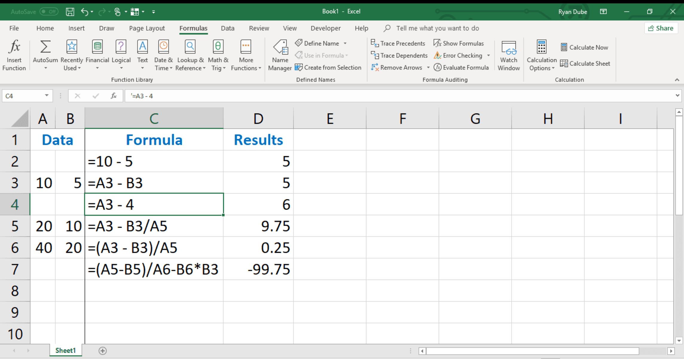
To subtract two numbers in Excel, you can use a simple subtraction formula or function. Begin by selecting the cell where you want the result to appear. Start the cell with an equals sign (=), followed by the first number, the minus sign (-), and then the second number. For example, if you want to subtract 5 from 10, the formula would be “=10-5.”
Once you have entered the formula, press Enter to calculate the result. The cell will display the difference between the two numbers.
Excel also allows you to directly subtract numbers within a cell. To do this, type the numbers with the minus sign in the cell, such as “-5.” Excel will recognize this as a negative number and treat it accordingly in calculations.
If you need to subtract more than two numbers, you can expand the formula by including additional minus signs and numbers. For example, “=10-5-3” would subtract 5 and 3 from 10, resulting in a value of 2 in the cell.
Keep in mind that Excel follows the usual mathematical rules of operation. It performs subtraction from left to right, so if you have a more complex equation, it is essential to use parentheses to ensure the desired order of operations.
Basic subtraction in Excel is a valuable tool for performing quick calculations and manipulating numerical data. By understanding the formula syntax and utilizing Excel’s built-in functions, you can efficiently subtract numbers and streamline your spreadsheet operations.
Subtracting Two Numbers
Subtracting two numbers in Excel is a fundamental operation that can be done using simple formulas or functions. In this section, we will explore the steps to subtract two numbers in Excel.
To subtract two numbers, first, select the cell where you want the result to appear. Begin the cell with an equals sign (=) followed by the first number, a minus sign (-), and then the second number. For example, if you want to subtract 8 from 15, the formula would be “=15-8”.
After entering the formula, press Enter on your keyboard. Excel will calculate the difference and display the result in the selected cell.
If the numbers you want to subtract are in separate cells, you can directly reference those cells in your formula. For example, if the first number is in cell A1 and the second number is in cell B1, the formula would be “=A1-B1”. Excel will subtract the value in cell B1 from the value in cell A1 and display the result.
It’s important to note that when subtracting numbers in Excel, the operation follows the usual mathematical rules. If the result of the subtraction is negative, Excel will display the negative value accordingly.
Additionally, Excel allows you to subtract numbers within a single cell by typing the numbers with a minus sign, such as “-5”. The minus sign tells Excel to treat the number as negative. However, this method is generally used for shorter calculations or when working on a single-cell basis.
By mastering the process of subtracting two numbers in Excel, you can efficiently perform mathematical operations and manipulate numerical data in your spreadsheets.
Subtracting More than Two Numbers
Excel provides the flexibility to subtract more than two numbers in a single calculation. Whether you have a list of expenses or need to calculate the total reduction in sales, Excel’s functionality can make subtracting multiple numbers a breeze. In this section, we will explore how to subtract more than two numbers in Excel.
To subtract more than two numbers, you can utilize the subtraction formula or function in Excel. Start by selecting the desired cell where you want the result to appear. Begin the cell with an equals sign (=) followed by the first number. Then, use the minus sign (-) to subtract each additional number, separating the numbers with dashes. For instance, if you want to subtract 5, 3, and 2 from 10, the formula would be “=10-5-3-2”.
After entering the formula, press Enter on your keyboard to calculate the result. Excel will display the final value, which is the subtraction of all the numbers.
If the numbers you want to subtract are in separate cells, you can directly reference those cells in your formula. Simply use the cell references instead of the actual numbers. For example, if the numbers you want to subtract are in cells A1, A2, A3, and A4, the formula would be “=A1-A2-A3-A4”.
When subtracting more than two numbers, it is essential to pay attention to the order of operations. Excel performs the subtraction from left to right, so if you want to prioritize certain calculations, you can use parentheses to specify the order. For example, to subtract 10 from 20 and then subtract 5 from the result, you would use the formula “=20-(10-5)”.
By utilizing Excel’s functionality to subtract more than two numbers, you can efficiently analyze data and perform calculations, saving time and effort in your spreadsheet tasks.
Subtracting Negative Numbers
In Excel, subtracting negative numbers follows the same principles as subtracting positive numbers. However, it is essential to pay attention to certain details to ensure accurate calculations. In this section, we will explore how to subtract negative numbers in Excel.
When subtracting a negative number in Excel, you can use either the subtraction formula or function. Start by selecting the desired cell where you want the result to appear. Begin the cell with an equals sign (=) followed by the first number. Then, use the minus sign (-) to subtract the negative number. For example, if you want to subtract -5 from 10, the formula would be “=10-(-5)”.
After entering the formula, press Enter on your keyboard to calculate the result. Excel will correctly subtract the negative number and display the final value.
Another approach to subtracting negative numbers in Excel is to use parentheses. Instead of a double negative sign, you can enclose the negative number within parentheses. The formula would be “=10-(5)”. This method can help eliminate confusion and improve readability when dealing with multiple negative numbers.
It’s important to note that if you only input a negative number without any subtraction operator (such as “-5”), Excel will automatically treat it as a negative value. However, if you include a minus sign before a positive number (such as “-5” in a cell), Excel will interpret it as a negative value as well.
When subtracting negative numbers in Excel, be mindful of maintaining the correct order of operations. Utilize parentheses if necessary to ensure that the subtraction is performed in the desired sequence.
By understanding the nuances of subtracting negative numbers in Excel, you can confidently perform calculations involving both positive and negative values, allowing for accurate data analysis and financial tracking.
Using Subtraction Formula
In Excel, the subtraction formula is a simple and effective way to subtract numbers and calculate the difference between them. Whether you are subtracting two numbers or a series of numbers, understanding how to use the subtraction formula can streamline your calculations. In this section, we will explore how to use the subtraction formula in Excel.
To use the subtraction formula, select the cell where you want the result to appear. Begin the cell with an equals sign (=) followed by the first number. Then, use the minus sign (-) to indicate subtraction and enter the second number. For example, if you want to subtract 7 from 15, the formula would be “=15-7”.
After entering the formula, press Enter on your keyboard to calculate the result. Excel will perform the subtraction and display the difference in the selected cell.
When working with the subtraction formula, you can also refer to cell references instead of entering the actual numbers in the formula. This allows you to perform calculations dynamically based on changing values. For instance, if the numbers you want to subtract are in cells A1 and B1, the formula would be “=A1-B1”. Excel will automatically update the result if the values in A1 or B1 change.
Additionally, you can expand the use of the subtraction formula to subtract more than two numbers. Simply add additional minus signs and numbers to the formula. For example, if you want to subtract 5, 3, and 2 from 10, the formula would be “=10-5-3-2”. Excel will process the subtraction operations from left to right and display the final result.
Using the subtraction formula in Excel provides a versatile and powerful way to perform subtraction calculations. By understanding the formula syntax and utilizing cell references, you can efficiently subtract numbers and manipulate data throughout your spreadsheets.
Using Subtraction Function
In addition to the subtraction formula in Excel, you can also utilize the subtraction function to subtract numbers and calculate the difference between them. The subtraction function provides a more structured approach to performing subtraction calculations, especially when dealing with a large number of values. In this section, we will explore how to use the subtraction function in Excel.
To use the subtraction function, select the cell where you want the result to appear. Begin the cell with an equals sign (=) followed by the word “SUBTRACT”. Then, within parentheses, enter the first number, followed by a comma (,), and then the second number. For example, if you want to subtract 7 from 15, the function would be “=SUBTRACT(15,7)”.
After entering the function, press Enter on your keyboard to calculate the result. Excel will perform the subtraction using the specified numbers and display the difference in the selected cell.
The subtraction function in Excel is not limited to subtracting only two numbers. You can expand the function to subtract more than two numbers by extending the list of arguments separated by commas. For instance, to subtract 5, 3, and 2 from 10, the function would be “=SUBTRACT(10,5,3,2)”. Excel will subtract all the specified numbers and display the final result.
When using the subtraction function, you can also refer to cell references as arguments instead of entering the numbers directly. This allows for dynamic calculations that update automatically when the values in the referenced cells change.
By using the subtraction function in Excel, you can perform complex subtraction operations with ease. It provides a structured approach to handling multiple numbers and offers flexibility for dynamic calculations, enhancing the accuracy and efficiency of your spreadsheet tasks.
Subtracting Numbers in Different Cells
Excel allows you to subtract numbers that are located in different cells within your worksheet. Whether you want to subtract numbers from different columns or different rows, Excel provides a flexible approach to perform these calculations. In this section, we will explore how to subtract numbers in different cells in Excel.
To subtract numbers in different cells, select the cell where you want the result to appear. Begin the cell with an equals sign (=) followed by the cell reference of the first number. Then, use the minus sign (-) to indicate subtraction and enter the cell reference of the second number. For example, if you want to subtract the value in cell A1 from the value in cell B1, the formula would be “=B1-A1”.
After entering the formula, press Enter on your keyboard to calculate the result. Excel will subtract the value in cell A1 from the value in cell B1 and display the difference in the selected cell.
You can apply the same approach to subtract numbers from different columns. For instance, if you want to subtract the value in cell C1 from the value in cell E1, the formula would be “=E1-C1”. Excel will perform the subtraction operation and show the result in the chosen cell.
When subtracting numbers from different rows, follow a similar process. For instance, if you want to subtract the value in cell A2 from the value in cell A5, the formula would be “=A5-A2”. Excel will calculate the difference and display the result accordingly.
By referencing different cells in your subtraction formula, you can perform calculations that involve numbers located in various parts of your worksheet. This allows for greater flexibility and accuracy when analyzing data and performing mathematical operations in Excel.
Subtracting Numbers in the Same Cell
In Excel, you can also subtract numbers within the same cell, which can be useful for performing quick calculations or manipulating data without the need for separate cells. This feature allows you to write a single formula that subtracts numbers within a cell, saving time and simplifying your spreadsheet. In this section, we will explore how to subtract numbers in the same cell in Excel.
To subtract numbers in the same cell, simply type the numbers with the minus sign directly into the cell. For example, if you want to subtract 5 from 10, you can enter “-5” in the cell.
Excel recognizes this as a negative number and performs the subtraction operation accordingly. When you press Enter, Excel will display the result, which is the difference between the numbers you entered.
If you need to subtract multiple numbers within the same cell, you can utilize the minus sign to separate the numbers. For instance, if you want to subtract 3, 2, and 1 from 10, you can enter “-3-2-1” in the cell. Excel will calculate the result by subtracting each number in the sequence.
By subtracting numbers in the same cell, you can streamline your calculations and eliminate the need for creating additional cells. This feature comes in handy when working on smaller calculations or when space is limited in your spreadsheet.
It’s important to note that when subtracting numbers in the same cell, Excel treats the entry as a text string rather than a number. Therefore, if you plan to use the result in further calculations or analyses, you may need to convert the text string back into a numeric value using the appropriate Excel functions.
By leveraging the ability to subtract numbers within the same cell, you can efficiently perform calculations and manipulate data in Excel, allowing for increased productivity in your spreadsheet tasks.
Subtracting Numbers in Different Worksheets or Workbooks
Excel offers the ability to subtract numbers that are located in different worksheets or even separate workbooks. This functionality allows you to perform calculations across multiple sheets or files, providing a comprehensive approach to data analysis and manipulation. In this section, we will explore how to subtract numbers in different worksheets or workbooks in Excel.
To subtract numbers from different worksheets or workbooks, start by selecting the cell where you want the result to appear. Begin the cell with an equals sign (=) followed by the sheet name or workbook reference where the number is located. Use an exclamation mark (!) to separate the sheet name or workbook reference from the cell reference. Then, enter the cell reference that contains the first number. Next, use the minus sign (-) to indicate subtraction and enter the cell reference that contains the second number. For example, if you want to subtract the value in cell A1 from Sheet2 in Cell A1 from Sheet1, the formula would be “=Sheet1!A1-Sheet2!A1”.
After entering the formula, press Enter on your keyboard to calculate the result. Excel will subtract the value in the specified cell in Sheet2 from the value in the specified cell in Sheet1 and display the difference in the selected cell.
You can apply the same concept when subtracting numbers from different workbooks. Begin the cell with an equals sign (=) followed by the workbook reference in square brackets ([ ]). Enter the sheet name, exclamation mark, and the cell reference for the first number. Then, use the minus sign (-) to indicate subtraction and enter the sheet name, exclamation mark, and cell reference for the second number.
By referencing numbers in different worksheets or workbooks, you can perform calculations that span multiple data sources. This feature is particularly useful when analyzing data from various sources or consolidating information from different collaborators.
Keep in mind that when referencing cells in different worksheets or workbooks, it’s crucial to ensure that the referenced files or sheets are open and accessible to Excel. Otherwise, Excel will display an error or a value that doesn’t match your expectations.
By leveraging the ability to subtract numbers from different worksheets or workbooks, you can perform comprehensive calculations and data analysis in Excel, allowing for a more thorough examination and interpretation of your data.
Using Autofill for Subtraction
Excel’s Autofill feature is a time-saving tool that allows you to quickly and easily subtract numbers in a series or pattern. Whether you need to subtract numbers sequentially or create a pattern of subtracted values, Autofill can streamline the process for you. In this section, we will explore how to use Autofill for subtraction in Excel.
To use Autofill for subtraction, begin by entering the first subtracted value in a cell. Then, select the cell and hover your mouse cursor over the bottom-right corner until it changes to a small black “+” symbol. Click and drag the mouse down or across, depending on the desired direction, to apply the subtraction pattern.
As you drag, Excel will automatically fill in the subsequent cells with the subtracted values based on the pattern you established. For example, if the first subtracted value is in cell A1 and you drag the mouse cursor down, Excel will subtract the same amount from the corresponding cells in column A.
If you have a specific pattern or sequence in mind, you can establish it by entering the first few subtracted values manually. Once you have this pattern set, select the cells containing the pattern and drag the Autofill handle to continue the subtraction pattern.
Autofill can also intelligently generate a subtraction pattern based on a series of existing numbers. For instance, if you have a series of numbers in column A and want to create a corresponding column of subtracted values, select the first cell in column B where you want the subtracted values to appear. Then, drag the Autofill handle across the adjacent cells. Excel will automatically calculate the difference between the corresponding cells in column A and fill in the subtracted values in column B.
By using Autofill for subtraction, you can quickly generate a series or pattern of subtracted values without the need for manual input. This feature is particularly useful when working with large datasets or when you need to create a sequential or patterned list of subtracted values.
Remember to double-check the results after applying Autofill, especially when working with complex patterns or formulas. This ensures the accuracy of your subtracted values and maintains data integrity.
Utilizing the Autofill feature for subtraction can significantly speed up your data manipulation and calculation processes in Excel, allowing for more efficient spreadsheet management.
Using Absolute Cell References in Subtraction
Excel provides a powerful feature called absolute cell references, which allows you to fix specific cells in a subtraction formula. By using absolute cell references, you can ensure that certain cells remain constant while subtracting values from other cells that change. In this section, we will explore how to use absolute cell references in subtraction formulas in Excel.
To use absolute cell references in a subtraction formula, you should use a dollar sign ($) before the column letter and/or row number of the cell you want to fix. This dollar sign signifies that the referenced cell should remain constant and not adjust when the formula is copied or filled. Here’s how to use it:
1. Start by selecting the cell where you want the result of the subtraction to appear.
2. Begin the cell with an equals sign (=) followed by the subtraction formula.
3. Use the dollar sign ($) before the column letter and/or row number of the cell(s) you wish to fix.
4. Enter the cell reference(s) for the numbers you want to subtract in the formula, using relative references for the changing cells.
For example, consider the scenario where you want to subtract the value in cell A1 from all the values in column B. The subtraction formula with an absolute cell reference would look like this: “=$A$1-B1”. As you copy or fill the formula down the column, the value in cell A1 remains constant, while the value in column B updates accordingly.
Alternatively, if you want to subtract a fixed value from different cells, you can use an absolute cell reference for the value you want to subtract. For instance, if you want to subtract the value in cell C1 from all the values in column D, the formula would be “=D1-$C$1”. In this case, the value in cell C1 remains constant while the formula adjusts for each cell in column D.
By using absolute cell references, you can ensure that specific cells are always included or excluded from the subtraction operation, regardless of how the formula is copied or filled. This is particularly useful when working with complex datasets or formulas that involve fixed reference points.
Remember to be careful when copying or filling formulas with absolute cell references. Ensure that the referenced cells align correctly with your intended calculations to avoid errors or inaccuracies.
Utilizing absolute cell references in subtraction formulas provides greater control and accuracy in your calculations, allowing for more efficient data analysis and manipulation in Excel.
Troubleshooting Subtraction Errors
While working with subtraction formulas in Excel, you may encounter various errors that can impact the accuracy of your calculations. Fortunately, Excel provides helpful error messages and tools to troubleshoot and resolve these issues. In this section, we will explore common subtraction errors and techniques for troubleshooting them in Excel.
1. #VALUE! Error: This error typically occurs when one or both of the cells in the subtraction formula contain non-numeric values. Double-check the cells and ensure that they contain valid numbers or use the ISNUMBER function to verify the value’s data type before subtracting.
2. #DIV/0! Error: This error appears when you attempt to divide a value by zero. Check if any of the cells involved in the subtraction have a value of zero or use an IF statement to handle the division-by-zero scenario gracefully.
3. #REF! Error: The #REF! error occurs when the formula references a cell or range that has been deleted, moved, or no longer exists. Double-check the cell references in your subtraction formula and ensure they are valid.
4. #NUM! Error: This error indicates an invalid numeric value. It can occur if the subtraction results in a value that exceeds the allowed numeric range or if the formula contains invalid mathematical operations. Review your formula and ensure all calculations are valid.
5. Incorrect results: If you are getting unexpected or incorrect results, check for any discrepancies in your formula, such as incorrect cell references, missing parentheses, or misplaced operators. Double-check the order of operations and consider using additional parentheses to clarify the intended calculation order.
6. Inconsistent formatting: Sometimes, the formatting of cells involved in the subtraction may cause issues, resulting in incorrect or unexpected results. Ensure that the cells have consistent number formatting and that they are formatted as numeric values and not text.
If you encounter subtraction errors in Excel, consider using the Evaluate Formula feature to analyze your formula step by step. This tool can help identify the specific point of error and guide you towards a solution.
Additionally, take advantage of Excel’s built-in help resources and community forums for specific error messages. These resources can provide insights and solutions to common subtraction errors that you may encounter.
By understanding the common subtraction errors and utilizing Excel’s troubleshooting tools, you can effectively address and resolve issues, ensuring accurate subtraction calculations in your spreadsheets.