
Overview of Google Spreadsheets
Google Spreadsheets is a powerful cloud-based spreadsheet application that offers a wide range of features for organizing, analyzing, and manipulating data. It provides a user-friendly interface and collaborative capabilities, making it an excellent tool for personal and professional use. Whether you’re managing financial data, tracking project progress, or creating charts and graphs, Google Spreadsheets has got you covered.
One of the key advantages of using Google Spreadsheets is its accessibility. Since it is web-based, you can access your spreadsheets from any device with an internet connection. This enables real-time collaboration with team members, making it easy to work on spreadsheets together, from different locations.
Google Spreadsheets offers a wide range of templates to help you get started quickly. Whether you’re creating a budget, a schedule, or a sales report, you can choose from various pre-built templates that are customizable to suit your specific needs. Additionally, you can import data from other sources such as CSV files or Microsoft Excel, making it simple to migrate your existing spreadsheets to Google Spreadsheets.
The application provides a variety of functions and formulas that allow you to perform complex calculations and data manipulations. Whether you need to add up numbers, find averages, or calculate percentages, Google Spreadsheets has functions like SUM, AVERAGE, and PERCENTAGE that make these tasks effortless.
Moreover, Google Spreadsheets offers data visualization tools, such as charts and graphs, which allow you to present your data in a visually appealing manner. Whether you prefer bar charts, pie charts, or line graphs, you can select from various types of charts and customize them to convey your data effectively.
Collaboration is at the core of Google Spreadsheets. You can invite others to collaborate on your spreadsheets, assign different levels of permissions, and track changes made by collaborators. This makes it easy to work on spreadsheets with your team, review and provide feedback, and ensure that everyone is on the same page.
Understanding Rounding in Google Spreadsheets
Rounding numbers is a common task in data analysis and financial calculations. In Google Spreadsheets, rounding can be achieved through various formulas and functions, each with its own purpose and method. Understanding the different rounding options available in Google Spreadsheets is essential to ensure accurate results in your calculations.
The most commonly used rounding function in Google Spreadsheets is the ROUND function. This function allows you to round a number to a specified number of decimal places. For example, if you want to round a number to two decimal places, you would use the formula =ROUND(A1, 2), where A1 is the cell containing the number you want to round. The ROUND function follows standard rounding rules, rounding up if the next digit is 5 or greater.
In certain situations, you may need to round numbers up to the nearest whole number or a specific multiple. For these scenarios, Google Spreadsheets provides the CEILING function. This function rounds numbers up towards positive infinity. For example, if you want to round a number up to the nearest whole number, you would use the formula =CEILING(A1, 1). The CEILING function can also be used to round numbers up to the nearest multiple. For instance, to round a number up to the nearest multiple of 10, you would use the formula =CEILING(A1, 10).
Another useful rounding function in Google Spreadsheets is the INT function. This function rounds a number down to the nearest whole number. For example, if you want to round a number down to the nearest whole number, you would use the formula =INT(A1).
If you specifically need to round numbers up, regardless of the decimal value, you can use the ROUNDUP function. This function always rounds numbers up to the nearest whole number or the specified number of decimal places. For instance, to round up a number to the nearest whole number, you would use the formula =ROUNDUP(A1, 0).
In some cases, you may want to round numbers up to a specified multiple, rather than a whole number. This can be achieved using the MROUND function. With this function, you can round numbers up or down to the nearest specified multiple. For example, if you want to round a number up to the nearest multiple of 5, you would use the formula =MROUND(A1, 5).
Lastly, you can also create your own rounding formula using the ROUND function combined with other functions or mathematical operations. This gives you full flexibility and control over how numbers are rounded in your spreadsheet.
Understanding the different rounding functions in Google Spreadsheets allows you to efficiently perform calculations and ensure accurate results in your spreadsheets. By using the appropriate rounding method for your specific needs, you can effectively manage and analyze your data with confidence.
Using the ROUND function
The ROUND function in Google Spreadsheets is a versatile tool for rounding numbers to a specified number of decimal places. With this function, you can ensure that your calculations are precise and aligned with your desired level of precision.
The syntax of the ROUND function is simple. It takes two arguments: the number you want to round and the number of decimal places to round to. For example, if we have a number in cell A1 that we want to round to two decimal places, the formula would be =ROUND(A1, 2).
It’s important to note that the ROUND function follows standard rounding rules. If the next digit after the specified decimal places is 5 or greater, the number is rounded up. If the next digit is less than 5, the number is rounded down.
Here’s an example to illustrate the usage of the ROUND function. Let’s say you have a column of numbers representing product prices, and you want to round them to the nearest dollar. Using the ROUND function, you can achieve this quickly and efficiently. In an empty column, you can enter the formula =ROUND(A1, 0), where A1 is the cell containing the original price. This will round the price to the nearest whole dollar.
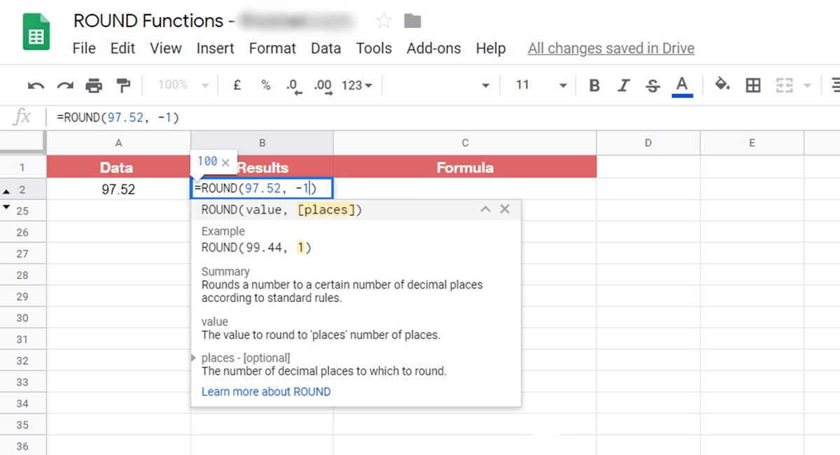
In addition to rounding numbers to a specified number of decimal places, the ROUND function can also be used to round numbers to negative decimal places. This can be useful when you want to round numbers to the nearest ten, hundred, or thousand. For example, if you have a number in cell A1 that you want to round to the nearest hundred, you can use the formula =ROUND(A1, -2).
It’s worth mentioning that the ROUND function can be combined with other functions and formulas to achieve more advanced rounding scenarios. For instance, you can use the ROUND function within an IF statement to round numbers based on specific conditions.
Using the ROUND function in Google Spreadsheets provides you with the flexibility to control the precision of your calculations. Whether you need to round numbers to specific decimal places or to the nearest whole number, the ROUND function offers a simple and effective solution.
Rounding numbers up with the CEILING function
When you need to round numbers up to the nearest whole number or a specific multiple, the CEILING function in Google Spreadsheets comes in handy. This function allows you to round numbers up towards positive infinity, ensuring that your calculations reflect the desired level of precision.
The syntax of the CEILING function is straightforward. It requires two arguments: the number you want to round and the significance or multiple to which you want to round up. For example, if you have a number in cell A1 that you want to round up to the nearest whole number, the formula would be =CEILING(A1, 1).
The CEILING function not only rounds numbers up to the nearest whole number but also allows you to round numbers up to a specified multiple. For instance, if you have a series of numbers in column A representing quantities that need to be rounded up to the nearest multiple of 5, you can use the formula =CEILING(A1, 5) in an adjacent column to achieve this. The CEILING function will round each number up to the nearest whole multiple of 5.
It’s important to note that the CEILING function rounds numbers up, regardless of the decimal value. Therefore, if the number is already a whole number or an exact multiple, the function will leave it unchanged. It will only affect numbers that have a decimal component.
Another useful feature of the CEILING function is that you can use negative significance values to round numbers up to the nearest ten, hundred, or thousand. For example, if you have a number in cell A1 that you want to round up to the nearest hundred, you can use the formula =CEILING(A1, -2).
The CEILING function can be combined with other functions and formulas to perform more complex rounding calculations. For example, you can nest the CEILING function inside an IF statement to conditionally round numbers based on specific criteria.
Using the CEILING function in Google Spreadsheets allows you to conveniently round numbers up to the nearest whole number or a specified multiple. Whether you need to round quantities, prices, or any other numerical data, the CEILING function provides a versatile solution for achieving accurate and precise results.
Rounding numbers up to the nearest specified multiple with the CEILING function
When working with numbers in Google Spreadsheets, there are often instances where you need to round numbers up to a specific multiple. This can be useful in various scenarios, such as calculating quantities, adjusting prices, or any situation where values need to be aligned to a specific interval. In Google Spreadsheets, you can accomplish this rounding task using the CEILING function.
The CEILING function allows you to round numbers up to the nearest specified multiple. It takes two arguments—the number you want to round and the significance representing the multiple you want to round up to. For instance, if you have a number in cell A1 and you want to round it up to the nearest multiple of 5, you can use the formula =CEILING(A1, 5).
By using the CEILING function in this way, any number in cell A1 will be rounded up to the next multiple of 5. For example, if the value in A1 is 16, the formula will round it up to 20. Similarly, if the value is 23, the formula will round it up to 25.
It is important to note that the CEILING function rounds numbers up, regardless of their decimal value. Therefore, numbers that are already multiples of the specified value or whole numbers will be left unchanged. Only numbers with a decimal component will be rounded up to the nearest desired multiple.
The CEILING function can also handle negative significance values. This allows you to round numbers up to the nearest ten, hundred, or thousand. For example, if you have a value in cell A1 and you want to round it up to the nearest hundred, you can use the formula =CEILING(A1, -2).
By utilizing the CEILING function to round numbers up to the nearest specified multiple, you can ensure that your calculations align with the desired intervals or intervals mandated by external requirements. This functionality enhances the accuracy and precision of your spreadsheet calculations, especially in situations where rounding values is crucial to maintain consistency and relevance.
Rounding numbers up with the INT function
In Google Spreadsheets, you can round numbers up to the nearest whole number using the INT function. This function is particularly useful when you need to truncate the decimal portion of a number and obtain the next highest integer value.
The INT function takes a single argument—the number you want to round up. For example, if you have a number in cell A1 and you want to round it up to the nearest whole number, you can use the formula =INT(A1).
Unlike other rounding functions, such as ROUND or CEILING, the INT function simply removes the decimal portion of a number without considering the decimal value. This means that the result is always rounded down to the nearest whole number or integer value.
For instance, if the value in cell A1 is 3.86, the INT function will round it up to 4. Similarly, if the value is -2.25, the INT function will round it up to -2. It’s important to note that the INT function does not perform traditional rounding by considering the decimal value. Instead, it effectively truncates the decimal portion and moves towards zero.
The INT function has its limitations, as it only works for rounding up to the nearest whole number. If you need to round numbers up to a specific decimal place or a multiple, you will need to use other rounding functions like ROUND or CEILING.
Additionally, the INT function can be combined with other formulas and functions to create more complex rounding criteria. For example, you can use it within an IF function to conditionally round numbers up based on specific conditions. This enables you to customize the rounding process and achieve more sophisticated rounding outcomes.
By utilizing the INT function in Google Spreadsheets, you can easily round numbers up to the nearest whole number. Whether you need to round up quantities, calculate totals, or manipulate data, the INT function provides a simple and effective solution for your rounding needs.
Rounding numbers up with the ROUNDUP function
In Google Spreadsheets, the ROUNDUP function is a powerful tool for rounding numbers up to the nearest whole number or a specific decimal place. This function ensures that your calculations reflect a higher value, providing a more accurate representation of data.
The syntax of the ROUNDUP function is simple. It takes two arguments—the number you want to round up and the number of decimal places to round to. For example, if you have a number in cell A1 and you want to round it up to the nearest whole number, you can use the formula =ROUNDUP(A1, 0).
The ROUNDUP function always rounds numbers up, regardless of the decimal value. This means that if the value in cell A1 is 3.2, the ROUNDUP function will round it up to 4. Similarly, if the value is -2.6, the function will round it up to -3.
Aside from rounding up to the nearest whole number, the ROUNDUP function also allows you to round numbers up to a specific decimal place. For instance, if you want to round a number in cell A1 up to two decimal places, you can use the formula =ROUNDUP(A1, 2). This will result in the number being rounded up to the next highest two decimal places.
The ROUNDUP function can be particularly useful in financial calculations or situations where you need to ensure that values are rounded up to the next highest amount. For example, when calculating costs, prices, or payments, rounding up ensures that you have accounted for potential additional expenses.
It’s worth noting that the ROUNDUP function is always rounding numbers up, regardless of other factors. If you need more control over the rounding process, such as rounding numbers down or rounding based on specific conditions, you may need to use different rounding functions or incorporate the ROUNDUP function into more complex formulas.
By utilizing the ROUNDUP function in Google Spreadsheets, you can round numbers up to the nearest whole number or a specific decimal place. This functionality enhances the accuracy and precision of your calculations, ensuring that values accurately reflect the higher end of the rounding spectrum.
Rounding numbers up with the MROUND function
In Google Spreadsheets, the MROUND function is a useful tool for rounding numbers up or down to the nearest specified multiple. This function allows you to customize the rounding process and ensure that your calculations align with specific intervals or multiples.
The syntax of the MROUND function is straightforward. It requires two arguments—the number you want to round and the significance representing the desired multiple. For example, if you have a number in cell A1 and you want to round it up to the nearest multiple of 5, you can use the formula =MROUND(A1, 5).
The MROUND function rounds numbers up or down based on the specified multiple. If the decimal portion of the number is exactly halfway between two multiples, it is rounded to the nearest even multiple. For example, if the value in cell A1 is 7.5, using the formula =MROUND(A1, 2) will round it up to 8, as it is closer to the next even multiple of 2.
If you want to always round numbers up to the nearest multiple, regardless of the decimal value, you can combine the MROUND function with the CEILING function. For example, if you have a value in cell A1 and you want to always round it up to the nearest multiple of 5, you can use the formula =CEILING(A1, 5).
Conversely, if you want to always round numbers down to the nearest multiple, you can use the FLOOR function in combination with the MROUND function. For example, if you have a value in cell A1 and you want to always round it down to the nearest multiple of 10, you can use the formula =FLOOR(A1, 10).
The MROUND function provides flexibility in managing rounding scenarios, allowing you to align values with specific intervals or desired multiples. Whether you’re working with quantities, scores, or any type of numerical data, the MROUND function empowers you to round numbers up or down based on your specific needs.
It’s important to note that negative significance values can also be used with the MROUND function. This means you can round numbers up or down to the nearest negative multiple as well, such as -5, -10, or -100, depending on your requirements.
By utilizing the MROUND function in Google Spreadsheets, you can accurately round numbers up or down to the nearest specified multiple, offering greater precision and control over your data calculations.
Rounding numbers up with a formula and the ROUND function
In Google Spreadsheets, you can round numbers up to the nearest whole number or a specific decimal place by combining the ROUND function with a formula. This approach allows you to customize the rounding process and achieve precise results based on your specific requirements.
To round numbers up with a formula, you can utilize the ROUND function in conjunction with other functions or mathematical operations. The ROUND function takes two arguments—the number you want to round and the number of decimal places to round to.
For example, if you have a number in cell A1 and you want to round it up to the nearest whole number, you can use the formula =ROUND(A1, 0). This will effectively round the number up to the next highest integer.
If you want to round a number up to a specific decimal place, you can modify the second argument of the ROUND function. For instance, if you want to round a number to two decimal places, you can use the formula =ROUND(A1, 2). This will round the number up to the next highest value with two decimal places.
Now, to combine the ROUND function with a formula, you can include the desired formula or mathematical operation inside the first argument of the ROUND function. This allows you to perform calculations and immediately round the result up.
Let’s say you have a formula in cell A1 that calculates the average of a range of numbers. If you want to round up the average to the nearest whole number, you can use the formula =ROUND(AVERAGE(A1:A10), 0). This will calculate the average using the AVERAGE function and then round the result up to the next highest integer.
By using a formula in conjunction with the ROUND function, you have the flexibility to perform complex calculations and immediately round the result up, ensuring that your data reflects the desired level of precision and accuracy.
It’s important to note that when combining functions with the ROUND function, you need to consider the order of operations. Ensure that the formula is structured correctly to produce accurate results.
By employing the ROUND function within a formula, you can effectively round numbers up to the nearest whole number or a specific decimal place, providing you with precise results tailored to your specific needs.
Common mistakes when rounding numbers up
Rounding numbers up is a common task in data analysis and financial calculations. However, it is important to be aware of potential mistakes that can occur during the rounding process. These mistakes can lead to inaccurate results and compromise the integrity of your calculations. Here are some common mistakes to watch out for when rounding numbers up in Google Spreadsheets:
1. Rounding before final calculations: One common mistake is rounding numbers up too early in your calculations. It is best to perform all necessary calculations first and round the final result at the end of the process. Rounding prematurely can introduce rounding errors and affect the accuracy of your final outcome.
2. Rounding too aggressively: Another mistake is rounding numbers up to an unnecessary level of precision. Rounding to excessive decimal places can create an illusion of accuracy that may not be supported by the underlying data. It is important to consider the appropriate level of precision based on your specific needs and the nature of the data being rounded.
3. Neglecting negative numbers: Rounding negative numbers requires special attention. It is crucial to understand rounding rules and apply them correctly to negative values. For example, rounding -2.5 up to the nearest whole number may result in -2, rather than -3, depending on the rounding method used. Be aware of how rounding affects negative numbers in your calculations.
4. Ignoring significant figures: When working with significant figures, it is important to round numbers up while maintaining the appropriate number of significant figures. Rounding numbers too liberally can lead to loss of precision and inaccurate representation of the data. Be mindful of maintaining the correct number of significant figures throughout your calculations.
5. Rounding excessively large numbers: Rounding very large numbers can introduce significant errors if not handled carefully. When dealing with large numbers, consider whether rounding to a specific decimal place is necessary or if rounding to a whole number is sufficient for your analysis.
6. Failing to document rounding procedures: Lastly, it is essential to document the rounding procedures used in your calculations. This helps ensure transparency and reproducibility, and allows others to understand and verify your methodology. Documenting rounding procedures is especially important when sharing spreadsheets or when working collaboratively.
Awareness of these common mistakes and taking steps to avoid them will help you maintain accuracy and reliability in your rounding calculations. It is important to have a clear understanding of the rounding rules and to apply them appropriately in your analysis to ensure the integrity of your results.