Add The Current Date/Time In Excel Using Shortcut Keys

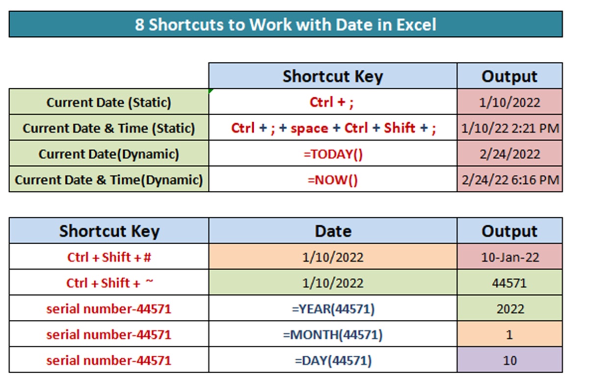
Method 1: Use the shortcut key Ctrl+; to add the current date

Adding the current date to an Excel spreadsheet can be quickly accomplished using a handy keyboard shortcut. By pressing Ctrl+; (semicolon), Excel will automatically insert the current date into the selected cell. This method is perfect when you need to add the date to a specific cell or as a reference point for ongoing work.

Using the Ctrl+; shortcut key provides a convenient way to insert the date without having to manually type it, reducing the risk of errors and saving you time. Whether you need to track project deadlines, record transactions, or simply keep a log of events, this keyboard shortcut will significantly streamline your data entry process.

To add the current date using this method, follow these simple steps:

1. Select the cell where you want to insert the date.
2. Press Ctrl+; (semicolon).
3. The current date will be instantly inserted into the selected cell.

By default, Excel will display the date in the format specified by your computer’s regional settings. However, you can customize the date format in Excel to match your specific requirements.

Using the Ctrl+; shortcut key for adding the current date is a powerful technique that can greatly improve your productivity when working with dates in Excel. Whether you’re a student, professional, or anyone who regularly deals with numbers and data, mastering this shortcut will undoubtedly make your life easier.

Method 2: Use the shortcut key Ctrl+Shift+; to add the current time

In addition to adding the current date, Excel offers a convenient shortcut for inserting the current time into a cell. By using the Ctrl+Shift+; (semicolon) keyboard combination, you can quickly input the current time, capturing it with precision for various time-tracking or timestamping purposes.

Here’s how you can leverage this shortcut to add the current time to your Excel spreadsheet:

1. Select the cell where you want to insert the time.
2. Press Ctrl+Shift+; (semicolon).
3. The current time will be immediately inserted into the selected cell, reflecting the exact time at the moment of insertion.

This efficient method eliminates the need to manually type the time, ensuring accuracy and saving you valuable time when working with time-sensitive data. Whether you’re managing schedules, tracking tasks, or analyzing data with time dependencies, using this shortcut will enhance your productivity and streamline your workflow.

Similar to the date shortcut, Excel will display the time in the format determined by your computer’s regional settings. However, you have the flexibility to customize the time format in Excel to meet your specific formatting requirements.

By mastering the Ctrl+Shift+; shortcut key, you can seamlessly incorporate the current time into your Excel worksheets, enhancing their functionality and keeping them up to date with accurate time information.

Method 3: Use the shortcut key Ctrl+Shift+: to add the current date and time together

If you need to capture both the current date and time in a single cell, Excel provides a convenient shortcut for that as well. By using the Ctrl+Shift+: (colon) keyboard combination, you can insert the current date and time together, providing a timestamp for time-sensitive data, logs, or event tracking.

To add the current date and time using this shortcut, follow these simple steps:

1. Select the cell where you want to insert the date and time.
2. Press Ctrl+Shift+: (colon).
3. The current date and time will be inserted into the selected cell, capturing the precise moment of insertion.

This shortcut is particularly useful when you need to track real-time data or record a specific event’s timestamp. By combining the date and time together, you can have a comprehensive record that accurately reflects when the event occurred without the need for separate date and time entries.

Like the other shortcuts, Excel will display the date and time format based on your computer’s regional settings. However, you have the flexibility to customize the display format according to your preferences or specific formatting requirements.

By using the Ctrl+Shift+: shortcut key, you can easily incorporate both the current date and time into your Excel worksheets, providing a complete timestamp for your records and facilitating efficient time tracking and analysis.

Method 4: Use the TODAY function to continuously update the date

If you need a dynamic date that updates automatically whenever you open or modify your Excel spreadsheet, the TODAY function is an excellent tool to achieve this. The TODAY function returns the current date, allowing you to keep your data up to date without manual intervention.

To use the TODAY function to continuously update the date in Excel, follow these steps:

1. Select the cell where you want the current date to appear.
2. Type “=TODAY()” (without the quotes) in the formula bar.
3. Press Enter.

The cell will now display the current date, and it will update accordingly every time you open or modify the spreadsheet. This feature is incredibly useful when you need to track progress over time, calculate durations, or perform time-based calculations.

The TODAY function is valuable in scenarios where you require real-time updates, such as project management, sales tracking, or financial analysis. It eliminates the need for manual adjustments and ensures that your data is always accurate and reflects the current date.

Since the TODAY function updates automatically, it’s essential to remember that the date will change each day, and the historical data will reflect the current date. If you need to capture fixed or static dates, consider using other methods or formulas in conjunction with the TODAY function.

By leveraging the TODAY function, you can effortlessly incorporate the current date into your Excel worksheets and enjoy the benefits of dynamic and accurate date tracking.

Method 5: Use the NOW function to continuously update the date and time

When you need to display both the current date and time in your Excel spreadsheet and have it automatically update as you work, the NOW function is the perfect solution. The NOW function returns the current date and time, allowing you to keep track of real-time information without constant manual updates.

To use the NOW function to continuously update the date and time in Excel, follow these steps:

1. Select the cell where you want the current date and time to appear.
2. Type “=NOW()” (without the quotes) in the formula bar.
3. Press Enter.

The cell will now display the current date and time, which will update automatically whenever you open or modify the spreadsheet. This feature is particularly useful for time-sensitive data, event tracking, or applications that require real-time information.

By using the NOW function, you can obtain accurate and up-to-date timestamps without the hassle of manual input. This function is invaluable in various scenarios, such as stock tracking, scheduling, or project management, where real-time data is crucial.

It’s important to note that the NOW function updates continuously, so each time you recalculate your sheet, the date and time will be refreshed. If you need to capture fixed or static timestamps, consider using other methods or formulas in combination with the NOW function.

With the NOW function at your disposal, you can effortlessly incorporate the current date and time into your Excel worksheets and ensure that your data is always precise and reflective of real-time information.

Method 6: Convert the date or time to a static value using Paste Special

While dynamic dates and times are useful in certain situations, there may also be instances where you want to convert them into static values to preserve a specific point in time. Excel’s Paste Special feature provides a simple and effective way to transform the current date or time into a fixed value.

To convert the date or time into a static value using Paste Special, follow these steps:

1. Select the cell containing the dynamic date or time.
2. Right-click on the selected cell, and choose “Copy” from the context menu, or use the keyboard shortcut Ctrl+C.
3. Right-click on a different cell where you want to paste the static value.
4. Select “Paste Special” from the context menu.
5. In the Paste Special dialog box, choose “Values” as the Paste option.
6. Click “OK” to apply the paste operation.

By following these steps, you effectively convert the dynamic date or time into a fixed value that won’t change with time or when the spreadsheet is recalculated. This is particularly useful when you want to preserve historic data or create a snapshot of a specific moment.

Converting dynamic dates or times into static values can help to maintain accurate records and prevent any unwanted changes or updates. It grants you control over the displayed time or date, which can be crucial for data analysis, reporting, or archiving purposes.

Keep in mind that once you convert the date or time to a static value, it will no longer update automatically. If you require real-time tracking, you should consider alternative methods, such as formulas or functions discussed in previous sections.

By utilizing the Paste Special feature to convert dynamic dates or times into static values, you can capture a specific instance and ensure the integrity of your data within your Excel spreadsheet.

Method 7: Customize the date and time format in Excel to suit your preferences

Excel provides a wide range of options for customizing the date and time formats to suit your specific needs and preferences. Whether you prefer a different date order, want to include leading zeros, or require a specific time format, Excel offers a flexible set of tools to make these adjustments.

To customize the date and time format in Excel, follow these steps:

1. Select the cell or range of cells containing the date or time.
2. Right-click on the selected cell(s), and choose “Format Cells” from the context menu.
3. In the Format Cells dialog box, navigate to the “Number” or “Custom” tab.
4. Select the desired date or time category from the list on the left.
5. Choose the format you prefer from the options on the right.
6. Click “OK” to apply the formatting changes.

By following these steps, you can modify the appearance of the dates and times in your spreadsheet, ensuring that they meet your specific requirements. Excel provides a wide variety of formats, such as short dates, long dates, time only, or a combination of both, allowing you to present the data in a visually appealing and easily understandable format.

Customizing the date and time format in Excel is particularly useful when working with international teams or when dealing with data from different regions that follow distinct date and time conventions. It also allows you to align your data presentation with the formatting standards of your organization or industry.

Furthermore, customizing the date and time format enhances data clarity and minimizes any confusion that may arise due to different date or time representations. It improves data interpretation and readability, making it easier to analyze and share information within your Excel spreadsheets.

By utilizing Excel’s flexible date and time formatting options, you can tailor the display of dates and times to your preferences, ensuring that your data is presented accurately and professionally.

Method 8: Use a keyboard shortcut to open the Format Cells dialog box and select the desired date and time format

Excel offers a convenient keyboard shortcut that allows you to quickly open the Format Cells dialog box and select the desired date and time format without navigating through the menus. This shortcut saves time and streamlines the process of formatting dates and times in your spreadsheet.

To use the keyboard shortcut to open the Format Cells dialog box and select the date or time format, follow these steps:

1. Select the cell or range of cells containing the date or time.
2. Press the keyboard shortcut Ctrl+1. (That’s the Ctrl key and the number one key simultaneously.)

This keyboard shortcut will instantly open the Format Cells dialog box, specifically to the “Number” tab, where you can select the desired date or time category and format. You can then navigate through the options using the arrow keys, choose the format you prefer, and press Enter to apply the formatting.

By using this keyboard shortcut, you eliminate the need to manually navigate through menus, saving you time and effort when formatting dates and times in your Excel spreadsheet. It provides a quick and efficient way to instantly access the formatting settings you need.

Customizing the date and time formats is particularly crucial when dealing with different regional conventions or specific presentation requirements. With this keyboard shortcut, you can easily experiment with different formats and choose the one that best suits your needs without interrupting your workflow.

Additionally, this shortcut is not just limited to formatting dates and times. It can be used to access the Format Cells dialog box for various other formatting options, such as number formatting or cell alignment. It is a versatile shortcut that enhances your overall formatting experience in Excel.

By utilizing the Ctrl+1 keyboard shortcut, you can swiftly open the Format Cells dialog box and customize the date and time formats to your liking, ensuring that your data is displayed accurately and aligns with your visual preferences.

Method 9: Combine the current date or time with other text in a cell using concatenation

Excel’s CONCATENATE function allows you to combine the current date or time with other text within a cell. This method is useful when you need to create a customized message, label, or timestamp that includes the current date or time alongside specific information or text.

To combine the current date or time with other text using concatenation, follow these steps:

1. Select the cell where you want to combine the date or time with text.
2. Type the desired text followed by an ampersand symbol (&).
3. For the current date, type “TODAY()” inside double quotation marks (“”).
4. For the current time, type “NOW()” inside double quotation marks (“”).
5. Press Enter to apply the formula and display the combined result.

For example, if you want to create a cell that displays “Today’s date is: [current date],” enter: “Today’s date is: ” & TODAY().

By using this concatenation technique, you can effortlessly incorporate the current date or time into your text, making it more dynamic and contextually relevant. This method is especially useful in scenarios where you need to generate personalized reports, labels, or messages that automatically update with the current date or time.

Furthermore, you can combine multiple text strings, including any desired separators or additional formatting, with the date or time function to create even more intricate and customized outputs. Excel’s concatenation feature opens up endless possibilities for manipulating and presenting your data.

Remember that the combined output will update dynamically with the current date or time whenever you recalculate the worksheet or open the file. If you need to freeze the value or preserve a specific timestamp, consider using other methods discussed earlier in this article.

By leveraging the power of concatenation in Excel, you can seamlessly combine the current date or time with other text to create dynamic and personalized cell contents, adding a new level of flexibility and customization to your spreadsheets.

Method 10: Use conditional formatting to highlight cells based on the current date or time

Conditional formatting in Excel allows you to dynamically highlight cells based on specific criteria. By utilizing this feature, you can easily highlight cells that contain the current date or time, creating visual cues and making important information stand out in your spreadsheet.

To use conditional formatting to highlight cells based on the current date or time, follow these steps:

1. Select the range of cells you want to apply the conditional formatting to.
2. Navigate to the “Home” tab in the Excel ribbon and click on the “Conditional Formatting” button.
3. In the dropdown menu, choose “New Rule.”
4. In the “New Formatting Rule” dialog box, select “Use a formula to determine which cells to format.”
5. Enter the appropriate formula based on your desired criteria. For example, to highlight cells with the current date, use the formula: =TODAY()=A1 (assuming A1 is the first cell in your selected range).
6. Customize the formatting options, such as font color, cell fill color, or borders, for the highlighted cells.
7. Click “OK” to apply the conditional formatting.

With conditional formatting, the specified range of cells will now be highlighted whenever the condition is met, indicating that they contain the current date or time. You can easily adjust the formatting criteria or expand the range to suit your specific requirements.

Conditional formatting offers a valuable way to visually identify and draw attention to important information, such as upcoming deadlines, time-sensitive data, or critical events. It enhances data interpretation and enables you to prioritize and analyze your spreadsheet more efficiently.

Furthermore, conditional formatting can be combined with other date or time-based rules to create more intricate formatting conditions. You can highlight cells that fall within a certain time range, automatically color-code entries based on their age, or implement various other formatting patterns to suit your needs.

By leveraging conditional formatting in Excel, you can easily highlight cells containing the current date or time, bringing focus to relevant information and making your data more visually appealing and accessible.

Method 11: Use the AutoFill feature to quickly populate a range of cells with the current date or time

Excel’s AutoFill feature is a powerful tool that allows you to automatically populate a range of cells with a series of values or patterns. Leveraging this feature, you can quickly fill cells with the current date or time, saving you time and effort when working with time-sensitive data.

To use the AutoFill feature to populate a range of cells with the current date or time, follow these steps:

1. Type the current date or time in a cell. For example, if you want to use the current date, type it in one cell.
2. Select the cell containing the current date or time and move your cursor to the bottom-right corner of the cell until it transforms into a thin crosshair (+).
3. Click and drag the crosshair down or across the range of cells where you want to populate the date or time.
4. Release the mouse button to apply the AutoFill and populate the selected range with the current date or time.

Excel will automatically increment or copy the original value in a pattern based on the selected cells’ relative positions. This feature allows you to efficiently fill multiple cells with sequential dates or times based on the initial value you entered.

The AutoFill feature is particularly useful when you have a uniform pattern of dates or times that need to be entered in a large range of cells. Instead of manually typing each value, you can rely on AutoFill to do the work for you. It saves time and minimizes the risk of errors.

Additionally, AutoFill can be used with various other date or time-related patterns. For example, you can fill a range with weekdays, specific intervals, or even custom date or time sequences by modifying the original value.

By utilizing the powerful AutoFill feature in Excel, you can effortlessly populate a range of cells with the current date or time. This method significantly accelerates the data entry process and ensures consistency and accuracy in your time-related data.

Method 12: Use the F9 key to manually update the date or time in a cell

Excel allows you to manually update the current date or time in a cell using the F9 key. This method is particularly useful when you want to capture a specific moment or need to refresh the displayed date or time without recalculating the entire spreadsheet.

To manually update the date or time in a cell using the F9 key, follow these steps:

1. Select the cell containing the date or time that you want to update.
2. Press the F9 key on your keyboard.

By pressing the F9 key, Excel recalculates the formula or function in the selected cell, updating the displayed date or time to the current values. This action allows you to obtain an instant refresh and confirm the most up-to-date information in your spreadsheet.

Using the F9 key is particularly useful when you have cells that contain formulas or functions referencing the current date or time. It enables you to verify the accuracy of your calculations and ensures that your data reflects the precise moment when the F9 key was pressed.

However, it’s important to note that using the F9 key on a range of cells may affect the entire workbook’s calculation process. If you want to manually update only specific cells, ensure that you have selected the appropriate range to avoid unintended consequences.

This manual update method is helpful in various scenarios, such as real-time monitoring, time-sensitive calculations, or verifying time-dependent formula results. It gives you full control over the refresh process without the need to recalculate the entire spreadsheet.

By utilizing the F9 key to manually update the date or time in a cell, you can refresh the displayed values and ensure the accuracy of time-related information in your Excel workbook.

Method 13: Add headers or footers with the current date or time to your Excel worksheet

Excel allows you to add headers or footers to your worksheets, which can include dynamic information such as the current date or time. This method is useful when you want to provide additional context to your worksheets or include a timestamp that updates automatically.

To add headers or footers with the current date or time to your Excel worksheet, follow these steps:

1. Go to the “Insert” tab in the Excel ribbon and click on the “Header & Footer” button.
2. In the header or footer section, select the location where you want to insert the date or time.
3. Click on the “Date” or “Time” button in the Header & Footer Design Tools.
4. Select the desired date or time format from the available options.
5. Click on “OK” to apply the changes to the header or footer.

By following these steps, Excel will automatically insert the current date or time in the selected header or footer section. This dynamic feature ensures that the date or time information will be updated every time you open or print the worksheet.

Adding headers or footers with the current date or time is helpful when you need to provide additional information, such as when the worksheet was last modified or printed. It enables you to maintain accurate timestamps and keep track of worksheet edits or versions.

Additionally, Excel allows you to customize the header or footer further, such as adding text, page numbers, or other worksheet-related information. You can combine dynamic elements like the date or time with static text to create comprehensive headers or footers that meet your specific needs.

Remember that headers and footers are visible in print layouts and when viewing the worksheet in Print Preview mode. They won’t be displayed in normal worksheet view, so it’s important to switch to the appropriate view to see and edit the headers or footers.

By incorporating headers or footers with the current date or time in your Excel worksheet, you can provide additional context, maintain accurate timestamps, and enhance the overall professionalism of your printed or shared documents.

Method 14: Use VBA code to add the current date or time in Excel

Excel’s Visual Basic for Applications (VBA) allows you to automate tasks and add custom functionality to your spreadsheets. Using VBA code, you can insert the current date or time into specific cells or perform actions based on time-related triggers. This method provides advanced flexibility and control over working with dates and times in Excel.

To use VBA code to add the current date or time in Excel, follow these steps:

1. Open the Visual Basic Editor by pressing Alt+F11 or navigating to the “Developer” tab and clicking on the “Visual Basic” button.
2. Insert a new module by right-clicking on the VBAProject (YourWorkbookName.xlsm) and selecting “Insert” > “Module.”
3. In the module, write the VBA code to add the date or time. For example, to insert the current date in cell A1, use the code: Range(“A1”).Value = Date.
4. Press F5 or click on the “Run” button in the toolbar to execute the code and insert the current date or time as specified.

VBA code provides extensive possibilities to manipulate dates and times in Excel. You can use it to perform calculations, generate dynamic reports, update cells based on specific conditions or events, and much more. It offers powerful automation capabilities, unlocking advanced functionality for your spreadsheets.

By utilizing VBA code, you can go beyond the limitations of built-in Excel functions and customize your date and time handling to suit your unique requirements. However, it’s important to have a basic understanding of VBA programming concepts to effectively implement and modify the code.

Keep in mind that VBA code execution is not automated by default in Excel. You need to manually execute the code or attach it to specific triggers or events for it to run automatically. This flexibility allows you to control when and how the date or time is added to your spreadsheet.

By incorporating VBA code into your Excel workflows, you can enhance the functionality and versatility of your worksheets. From basic date and time insertion to complex time-based automation, VBA empowers you to customize and optimize your Excel solutions.