
Understanding Gradient
Gradient plays a crucial role in machine learning algorithms, particularly in optimization techniques like gradient descent. To understand the concept of gradient, we need to delve into the realm of calculus. In calculus, the gradient represents the slope or rate of change of a function at a particular point.
In the field of machine learning, the gradient refers to the vector of partial derivatives of a multivariable function. It provides information about the steepness and direction of the function at a given point. The gradient can be imagined as a compass that guides us towards the direction where the function’s value increases the most rapidly.
By analyzing the gradient, machine learning models can identify the optimal values of parameters or coefficients that minimize a given cost or loss function. This process is crucial for training models effectively and accurately predicting outcomes.
Understanding the gradient allows us to harness its power to optimize machine learning models. When training a model, the gradient provides crucial information about the direction in which we should update the model’s parameters to minimize the loss function. By continuously updating the parameters in the direction opposite to the gradient, the model gradually converges towards the minimum point of the loss function.
Furthermore, gradient computation is an essential component in backpropagation, a fundamental algorithm for updating the weights and biases of neural networks during the training process. Backpropagation calculates the gradient of the loss function with respect to each parameter, making it possible to iteratively improve the model’s performance through successive iterations.
It is worth noting that the gradient can be positive, negative, or zero, indicating the direction in which the function increases, decreases, or remains constant, respectively. The magnitude of the gradient represents the steepness of the function.
In summary, the gradient is a fundamental concept in machine learning that enables optimization by providing information about the rate of change and direction of a function. By leveraging the gradient, models can iteratively update their parameters to minimize loss functions and improve performance.
The Role of Gradient in Machine Learning
The gradient plays a crucial role in machine learning algorithms, influencing various aspects of model training and optimization. From determining the direction of parameter updates to guiding the search for optimal solutions, the gradient serves as a compass in the vast landscape of machine learning.
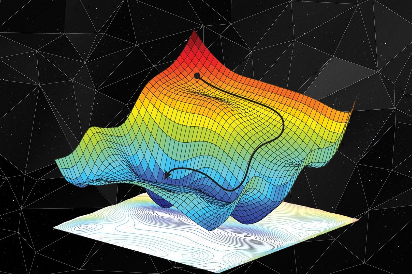
One of the primary roles of the gradient in machine learning is in optimization algorithms, particularly in the widely used technique called gradient descent. Gradient descent aims to find the global minimum of a cost or loss function by iteratively updating the model’s parameters in the opposite direction of the gradient. By following the gradient, the model can navigate through the parameter space, gradually approaching the optimal configuration that minimizes the loss function.
Moreover, the gradient enables models to adapt and learn from data. During the training phase, the model adjusts its parameters based on the gradient, which indicates how the loss function changes concerning each parameter. By computing the gradient, machine learning algorithms can learn the relationship between input features and target outputs, improving their predictive capabilities.
The gradient also plays a vital role in backpropagation, a central algorithm for training deep neural networks. Backpropagation calculates the gradient of the loss function with respect to every parameter in the network. This information is then used to update the weights and biases, enabling the model to learn hierarchical representations from the input data.
Furthermore, the gradient provides essential insights during the evaluation and fine-tuning of models. It can help identify regions of high utility in feature space and guide the selection of relevant features. By analyzing the gradient values, machine learning practitioners can gain a deeper understanding of the model’s behavior and make informed decisions about model improvements or adjustments.
In summary, the gradient plays a multifaceted role in machine learning. From facilitating optimization and parameter updates to enabling model adaptation and fine-tuning, the gradient is pivotal in the quest for accurate predictions and effective machine learning models. Understanding and leveraging the power of the gradient can lead to significant improvements in performance and the ability to tackle complex real-world problems.
Gradient Descent Algorithm
The gradient descent algorithm is an optimization technique widely used in machine learning for finding the optimal values of a model’s parameters. Its underlying principle is to iteratively update these parameters in the direction of the negative gradient of the cost function. By following this descent, the algorithm aims to reach the minimum point of the cost function and achieve the best possible fit to the data.
The gradient descent algorithm can be described in several steps. First, the process begins with initializing the parameters randomly or with predefined values. Then, the algorithm computes the gradient of the cost function with respect to each parameter using techniques such as backpropagation in neural networks. This provides information on the steepness and direction of the function at the current parameter values.
Next, the algorithm updates the parameters by taking a small step in the opposite direction of the gradient multiplied by a learning rate. The learning rate determines the size of the step and is crucial in balancing the convergence speed and stability of the algorithm. A low learning rate may result in slow convergence, while a high learning rate may lead to overshooting or instability.
This process of computing the gradient, updating the parameters, and iterating continues until a predefined stopping criterion is met. Common stopping criteria include reaching a maximum number of iterations or when the change in the cost function falls below a certain threshold.
There are different variations of the gradient descent algorithm, each with its own characteristics and advantages. The most basic form is called batch gradient descent, which computes the gradient and updates the parameters using the entire training dataset in each iteration. While this guarantees convergence, it can be computationally expensive for large datasets.
To address this issue, stochastic gradient descent (SGD) was introduced. SGD randomly selects a single training example or a small subset (mini-batch) at each iteration to compute the gradient and update the parameters. This makes the algorithm faster and more scalable, but it introduces some degree of noise in the parameter updates.
Another variant is the mini-batch gradient descent, which strikes a balance between batch gradient descent and SGD. It computes the gradient and updates the parameters using a randomly selected subset of the training data, providing a compromise between accuracy and efficiency.
In summary, the gradient descent algorithm is a fundamental optimization technique in machine learning. By iteratively updating the parameters in the opposite direction of the gradient, the algorithm aims to minimize the cost function and improve model performance. Understanding the different variations of gradient descent helps in selecting the most suitable algorithm for specific tasks and datasets.
Types of Gradient Descent Algorithms
Gradient descent, as a fundamental optimization technique in machine learning, has various variations that address specific challenges and trade-offs. Let’s explore some of the common types of gradient descent algorithms.
1. Batch Gradient Descent: This is the most basic form of gradient descent, where the algorithm computes the gradient and updates the parameters using the entire training dataset in each iteration. Batch gradient descent guarantees convergence to the global minimum but can be computationally expensive for large datasets.
2. Stochastic Gradient Descent (SGD): In contrast to batch gradient descent, SGD randomly selects a single training example or a small subset (mini-batch) at each iteration to compute the gradient and update the parameters. It is much faster and more scalable than batch gradient descent but introduces some degree of noise in the parameter updates.
3. Mini-Batch Gradient Descent: Mini-batch gradient descent strikes a balance between batch gradient descent and SGD. It computes the gradient and updates the parameters using a randomly selected subset of the training data. This approach provides a compromise between the accuracy of batch gradient descent and the efficiency of SGD. The mini-batch size can be adjusted based on the dataset size and computational resources.
4. Momentum-Based Gradient Descent: This variant of gradient descent helps to accelerate convergence by taking into account the past gradients. It introduces a momentum term that accumulates a fraction of the previous changes in the parameter updates. This momentum helps the algorithm to overcome local minima and plateaus by moving more quickly in consistent directions.
5. Nesterov Accelerated Gradient (NAG): Nesterov Accelerated Gradient is an extension of momentum-based gradient descent. It takes the momentum idea further by considering the future position of the parameters. Instead of using the current parameters to compute the gradient, it estimates the position the parameters will move to based on the momentum. NAG helps achieve faster convergence by allowing the algorithm to “look ahead” while computing the gradient.
6. Adagrad: Adagrad adjusts the learning rate of each parameter individually, based on the historical squared gradients. It scales down the learning rate for frequently updated parameters and scales up the learning rate for infrequently updated parameters. Adagrad is particularly useful in scenarios where the features have different frequencies in the dataset.
7. RMSprop: RMSprop, short for Root Mean Square Propagation, is an adaptive learning rate method that overcomes some limitations of Adagrad. RMSprop divides the learning rate by the exponentially decaying average of squared gradients. This helps to prevent the learning rate from diminishing quickly and smooths out the learning process.
These are just a few examples of the many types of gradient descent algorithms used in machine learning. Each algorithm offers unique properties and works well under specific circumstances. The choice of algorithm depends on factors such as the dataset size, computational resources, convergence speed, and desired trade-offs between accuracy and efficiency.
Advantages and Disadvantages of Gradient Descent
Gradient descent, as a widely used optimization technique in machine learning, offers several advantages and disadvantages. Understanding these pros and cons is crucial in leveraging the algorithm effectively for different tasks.
Advantages:
- Efficiency: Gradient descent algorithms, particularly stochastic and mini-batch gradient descent, are computationally efficient compared to batch gradient descent. They process only a subset of the training data in each iteration, making them suitable for large datasets and online learning scenarios.
- Scalability: Due to their smaller memory requirements and faster computation, stochastic and mini-batch gradient descent can handle large-scale machine learning tasks.
- Convergence: Gradient descent algorithms generally converge to a solution, finding parameters that minimize the cost function. Through careful tuning of the learning rate and regularization, it is possible to improve convergence speed and stability.
- Flexibility: Gradient descent algorithms can be applied to a wide range of machine learning models, including linear regression, logistic regression, and neural networks.
Disadvantages:
- Hyperparameter Sensitivity: Gradient descent algorithms require careful tuning of hyperparameters such as learning rate, mini-batch size, and regularization parameters. An incorrect choice of these hyperparameters can result in slow convergence, model instability, or failure to find the optimal solution.
- Local Minima: Gradient descent algorithms are susceptible to getting trapped in local minima, especially in complex high-dimensional spaces. However, with appropriate initialization and exploration strategies, it is possible to mitigate this issue.
- Noisy and Inconsistent Updates: Stochastic gradient descent, in particular, can introduce noise due to the random sampling of training examples. This noise can lead to inconsistent updates and a bumpy optimization path.
- Requires Sufficient Training Data: Gradient descent algorithms benefit from sufficient and representative training data. Insufficient or biased data can lead to suboptimal solutions or overfitting.
It is important to carefully consider these advantages and disadvantages when choosing and implementing gradient descent algorithms in machine learning projects. Through proper understanding and experimentation, the limitations can be mitigated and the algorithm’s strengths can be harnessed effectively.
Optimizing Gradient Descent
Gradient descent algorithms provide powerful optimization techniques for machine learning models. To improve their performance and address some of their limitations, several strategies and enhancements can be employed. Let’s explore some key approaches to optimizing gradient descent.
1. Learning Rate Optimization: The learning rate is a crucial hyperparameter in gradient descent algorithms. It determines the step size used to update the model’s parameters. Optimizing the learning rate is essential for achieving faster convergence and avoiding overshooting or oscillating around the minimum. Techniques like learning rate scheduling, adaptive learning rates (e.g., Adagrad, RMSprop, Adam), and learning rate decay can be used to improve the learning rate’s effectiveness.
2. Regularization Techniques: Regularization is useful for preventing overfitting and improving the generalization capacity of the model. Common regularization techniques include L1 and L2 regularization (ridge and lasso regularization), which add a penalty term to the cost function, encouraging the model to find simpler solutions with smaller parameter values. Regularization helps to prevent overemphasis on noisy or irrelevant features.
3. Batch Normalization: Batch normalization is a technique commonly used in deep neural networks to accelerate convergence and improve gradient flow. It normalizes the inputs to each layer by subtracting the batch mean and dividing by the batch standard deviation. This ensures that each layer receives inputs with similar scales, reducing the internal covariate shift problem and stabilizing the learning process.
4. Feature Scaling: Properly scaling the input features can significantly improve the performance of gradient descent. By normalizing or standardizing the input data, features with different scales or units are put on a comparable scale. This helps prevent the gradient from being dominated by features with larger magnitudes and improves the efficiency of the optimization process.
5. Exploratory Initialization: The choice of initial parameter values can have a significant impact on the convergence speed and final solution of gradient descent algorithms. Careful initialization, such as using small random weights or weights derived from pre-training, can help overcome local minima and initialize the optimization process in a more advantageous region of the parameter space.
6. Early Stopping: Monitoring the performance of the model on a validation set during training can help prevent overfitting. Early stopping is a technique where training is stopped when the performance on the validation set starts to degrade. This helps to find an optimal point along the convergence path, preventing the model from over-optimizing on the training data.
These are just a few of the many strategies for optimizing gradient descent algorithms. The specific techniques chosen will depend on the nature of the problem, the available data, and the complexity of the model. Experimentation and careful tuning are crucial to find the optimal combination of strategies that result in efficient and effective gradient descent optimization.
Common Issues and Challenges with Gradient Descent
While gradient descent is a powerful optimization algorithm, it is not without its challenges and issues. Understanding these common pitfalls is essential for successfully implementing and deploying gradient descent in machine learning projects. Let’s explore some of the most prevalent issues and challenges with gradient descent.
1. Local Minima: Gradient descent can sometimes converge to a local minimum instead of the desired global minimum of the cost function. Local minima are points in the parameter space where the cost function is locally minimized but not globally. Various strategies, such as using different initialization techniques and adding regularization, can help mitigate the impact of local minima.
2. Plateaus and Flat Areas: Plateaus and flat areas in the cost function can cause gradient descent to converge slowly. In these regions, the gradient becomes very small, making parameter updates minimal. Techniques such as momentum-based gradient descent or adaptive learning rates can alleviate this issue by keeping the update process more stable and avoiding stagnation on flat areas.
3. Vanishing or Exploding Gradients: For deep neural networks, the problem of vanishing or exploding gradients can occur during backpropagation. The gradients can become very small or very large, making it challenging to update the network’s parameters effectively. Techniques such as gradient clipping and using advanced optimization algorithms like RMSprop or Adam can help stabilize the gradient updates.
4. Overfitting: Gradient descent algorithms are susceptible to overfitting when the model becomes too complex and memorizes the training data instead of generalizing well to unseen data. Regularization techniques like L1 and L2 regularization can be used to combat overfitting by constraining the model’s complexity and reducing the influence of irrelevant features.
5. Hyperparameter Tuning: Proper tuning of hyperparameters, such as the learning rate, mini-batch size, and regularization parameter, is crucial for achieving optimal performance with gradient descent. Finding the right balance is often challenging and requires experimentation and iterative refinement.
6. Convergence Speed: Gradient descent algorithms may converge slowly, especially when dealing with large-scale datasets or highly complex models. Techniques like learning rate schedules, adaptive learning rates, and early stopping can be employed to speed up convergence and improve efficiency.
7. Curse of Dimensionality: As the number of features or parameters increases, gradient descent may suffer from the curse of dimensionality. The optimization landscape becomes more intricate, making it difficult for the algorithm to explore and find the global minimum. Careful feature selection and dimensionality reduction techniques can help mitigate this issue.
By being aware of these common challenges and issues, practitioners can proactively address them through careful hyperparameter tuning, appropriate initialization strategies, regularization techniques, and advanced optimization algorithms. Balancing complexity, computational resources, and the available dataset is key to overcoming these challenges and achieving optimal performance with gradient descent.
Applications of Gradient in Machine Learning
The concept of gradient has numerous applications across various domains in machine learning. It serves as a crucial component in optimization algorithms and enables efficient training and fine-tuning of models. Let’s explore some of the key applications of gradient in machine learning.
1. Model Training: The gradient guides the training process by indicating the direction and magnitude of parameter updates. Models learn from data by iteratively adjusting their parameters in the opposite direction of the gradient, improving their performance on the given task. Gradient descent algorithms, powered by the gradient, play a central role in training various machine learning models, including linear regression, logistic regression, and neural networks.
2. Neural Network Optimization: The backpropagation algorithm, a fundamental technique for training neural networks, relies heavily on the gradient. Backpropagation calculates the gradients of the loss function with respect to each parameter in the network. These gradients are then used to update the weights and biases, allowing the model to learn hierarchical representations from the input data. The efficient computation of gradients through backpropagation is critical for training deep neural networks.
3. Feature Selection: The gradient can be utilized to determine the importance or relevance of features in a machine learning model. By analyzing the gradient values associated with different features, practitioners can identify the most influential features and prioritize them during feature selection. This helps to streamline the model and improve its interpretability and performance.
4. Anomaly Detection: Gradients can also be leveraged for anomaly detection tasks. By computing the gradient of a model’s decision boundary or loss function, abnormal or outlier instances can be identified. Deviations from the expected gradient pattern indicate the presence of anomalies in the data, making gradient-based anomaly detection a valuable tool for various applications such as fraud detection and system monitoring.
5. Reinforcement Learning: In the field of reinforcement learning, the gradient plays a key role in policy optimization. Policy gradient methods utilize the gradient to iteratively update the policy parameters based on the performance feedback from the environment. These techniques allow agents to learn optimal policies through trial and error, maximizing long-term rewards in complex environments.
6. Generative Models: Generative models, such as generative adversarial networks (GANs) and variational autoencoders (VAEs), often rely on gradient-based optimization methods. These models learn to generate new samples by iteratively adjusting their parameters based on the gradient of a carefully designed objective function. The gradient guides the model’s learning process and enables the generation of realistic and novel samples.
7. Natural Language Processing: The gradient plays a significant role in training and fine-tuning language models for natural language processing tasks. Models such as recurrent neural networks (RNNs) and transformer-based architectures utilize gradient-based optimization to learn the intricate patterns and dependencies in textual data. The gradient helps models capture semantic relationships and generate coherent and meaningful outputs.
In summary, the gradient has diverse applications in machine learning. From training models and optimizing neural networks to feature selection and anomaly detection, the gradient serves as a fundamental tool for optimizing models and improving their performance in various domains. Embracing the power of the gradient enables practitioners to tackle complex problems and extract valuable insights from data.