What Is Gradient Boosting In Machine Learning

What Is Boosting?

Boosting is a popular machine learning technique that aims to improve the predictive accuracy of models by combining weak learners into a strong learner. It is a type of ensemble learning, where multiple models are trained to work together in order to achieve better performance than any individual model.

The key idea behind boosting is to iteratively train weak learners, such as decision trees or regression models, and focus on the samples that were incorrectly predicted in the previous iterations. By giving more weight to the misclassified samples, the subsequent weak learners can learn from the mistakes of the previous ones and improve the overall prediction accuracy.

Boosting algorithms are different from traditional methods like bagging, where each weak learner is trained independently. Instead, boosting assigns higher weights to misclassified samples and lower weights to correctly classified samples, allowing subsequent iterations to pay more attention to the misclassified samples and adjust the model accordingly. This process continues until a stopping criterion is met, or a predefined number of weak learners is reached.

Boosting has gained tremendous popularity in machine learning because of its ability to handle complex datasets and provide robust predictions. It has been successfully applied to various tasks, including classification, regression, and even ranking problems. Some well-known boosting algorithms include AdaBoost, Gradient Boosting, and XGBoost.

Boosting algorithms have proven to be highly effective in improving the performance of models, often achieving state-of-the-art results in many machine learning competitions and real-world applications. By combining the strengths of multiple weak learners, boosting is able to capture complex patterns in the data and make accurate predictions.

In the next section, we will delve into one specific type of boosting algorithm called Gradient Boosting and explore how it works in more detail.

How Does Gradient Boosting Work?

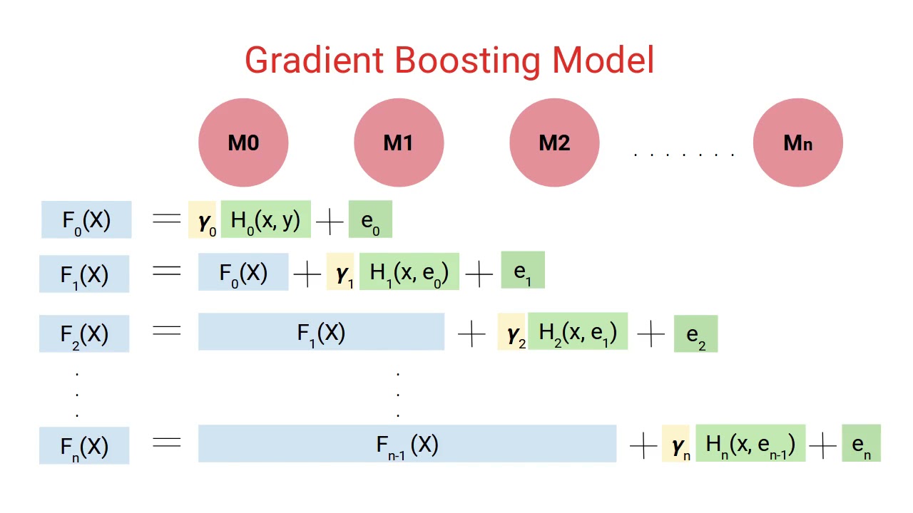
Gradient Boosting is a powerful machine learning algorithm that focuses on building an ensemble of weak prediction models in a sequential manner. It operates by minimizing a loss function through an optimization technique known as gradient descent.

The process of Gradient Boosting starts by initializing a model, which can be a simple decision tree with a single node. This initial model predicts the average value of the target variable for all the training samples. The difference between the actual target values and the predictions is known as the residual.

In each subsequent iteration, a new weak learner, referred to as a “base learner,” is trained to predict the residuals of the previous model. The base learner is usually a decision tree with a limited depth to avoid overfitting. The learning process involves adjusting the parameters of the base learner to minimize the loss function, which quantifies the difference between the predicted residuals and the true residuals.

After training the base learner, its predictions are multiplied by a predefined learning rate and added to the predictions of the previous model. This combination of predictions, called the “boosting step,” leads to an updated and more accurate prediction. The learning rate determines the contribution of each base learner to the final ensemble. A smaller learning rate makes the learning process more conservative, while a larger learning rate allows for faster learning but risks overfitting.

This iterative process continues until a stopping criterion is met, such as a maximum number of iterations or the desired performance metric is achieved. The final prediction is obtained by summing the predictions of all the models in the ensemble.

Gradient Boosting is particularly efficient in handling various types of data, including numerical, categorical, and missing values. It is also capable of capturing complex interactions and non-linear relationships in the data. These properties make it suitable for a wide range of machine learning tasks, such as regression, classification, and ranking.

Overall, Gradient Boosting stands out as a powerful and flexible algorithm due to its ability to iteratively improve model performance by focusing on the residuals of previous models. By combining the strengths of multiple weak learners, Gradient Boosting can achieve impressive predictive accuracy and outperform other traditional machine learning methods.

Advantages of Gradient Boosting

Gradient Boosting has gained popularity in the field of machine learning due to its numerous advantages and remarkable performance in various applications. Here are some key advantages of Gradient Boosting:

1. High Predictive Accuracy: Gradient Boosting is known for its ability to achieve high predictive accuracy by combining the predictions of multiple weak learners into a strong ensemble model. It is particularly effective in handling complex datasets with non-linear relationships and achieving state-of-the-art performance in various machine learning tasks.
2. Flexibility: Gradient Boosting can be applied to different types of data, including numerical, categorical, and missing values. This flexibility makes it suitable for a wide range of applications in diverse domains.
3. Handles Outliers: Gradient Boosting can effectively handle outliers in the data by assigning higher weights to misclassified samples during the training process. This helps to reduce the impact of outliers and improve the overall model’s robustness.
4. Feature Importance: Gradient Boosting provides a measure of feature importance, which helps in understanding the influence of different features on the final predictions. This information can assist in feature selection and feature engineering, leading to improved model performance.
5. Handles Missing Values: Gradient Boosting has built-in mechanisms to handle missing values in the dataset. It can handle missing values in both predictor variables and target variables, making it suitable for real-world datasets with incomplete or inconsistent data.
6. Interpretability: While Gradient Boosting is an ensemble model, it still provides some level of interpretability by allowing for the analysis of individual base learners. It is possible to examine the contribution and interactions of each base learner, providing insights into the decision-making process.
7. Regularization: Gradient Boosting incorporates regularization techniques, such as shrinkage and subsampling, which help in reducing overfitting and improving generalization performance. This allows for better handling of noise and variance in the data.

These advantages make Gradient Boosting a popular and powerful machine learning algorithm, capable of handling complex tasks and delivering accurate predictions. It is widely used in various domains, such as finance, healthcare, e-commerce, and more.

Understanding Decision Trees

Decision trees are fundamental components of Gradient Boosting and play a crucial role in the learning process. A decision tree is a hierarchical model that represents a series of decisions leading to a final prediction. Each internal node in the tree represents a decision based on a particular feature, while each leaf node represents the final prediction or outcome.

The construction of a decision tree involves recursively partitioning the data based on specific criteria. The goal is to create branches or splits that maximize the homogeneity or purity of the samples within each partition.

At each step, the decision tree algorithm selects the feature and threshold that lead to the best separation of the data. Different criteria for measuring the quality of a split can be used, such as Gini impurity or information gain. The chosen criterion evaluates how well a split separates the samples into different classes or groups.

Decision trees can handle both categorical and numerical features. For categorical features, the tree branches out based on the possible categories. For numerical features, the tree can make binary decisions based on whether the feature value exceeds a certain threshold or not.

One of the advantages of decision trees is their interpretability. The decision paths from the root to the leaf nodes can be easily understood and provide insights into the decision-making process. Additionally, decision trees can handle both classification and regression tasks, making them versatile for various types of problems.

However, decision trees tend to be highly sensitive to small changes in the training data, which can lead to overfitting. To address this issue, ensemble methods like Gradient Boosting use decision trees as weak learners and combine them in a sequential manner, allowing subsequent trees to correct the errors of the previous ones.

Furthermore, decision trees have limitations when it comes to capturing complex relationships and interactions in the data. They tend to be biased towards features that offer more splits early in the tree construction process. This is where Gradient Boosting’s iterative process helps, as subsequent trees can focus on the remaining patterns and improve the overall predictive power.

Overall, decision trees serve as the building blocks of Gradient Boosting, providing the base learners that are sequentially combined to improve model performance. Their interpretability and flexibility make them an essential component in understanding and extracting insights from the data.

Loss Functions in Gradient Boosting

Loss functions play a critical role in Gradient Boosting as they quantify the difference between the predicted values and the true values of the target variable. These functions guide the optimization process in each iteration, allowing the algorithm to learn and make more accurate predictions.

The choice of an appropriate loss function depends on the nature of the problem being addressed. There are different types of loss functions commonly used in Gradient Boosting, including:

1. Mean Squared Error (MSE): MSE is a commonly used loss function for regression problems. It computes the average squared difference between the predicted and true values of the target variable. Minimizing MSE leads to models that focus on reducing the overall variance in the predictions.
2. Mean Absolute Error (MAE): MAE is another loss function suitable for regression problems. It calculates the average absolute difference between the predicted and true values. Unlike MSE, MAE is less sensitive to outliers, making it more robust in the presence of extreme values.
3. Binary Cross-Entropy: Binary cross-entropy is used in binary classification problems where the target variable is binary. It measures the dissimilarity between the predicted probabilities and the true binary labels. The goal is to minimize the cross-entropy loss, which indicates a better alignment between the predicted probabilities and the actual classes.
4. Categorical Cross-Entropy: Categorical cross-entropy is employed in multiclass classification problems. It calculates the average cross-entropy loss across all classes. The aim is to minimize the discrepancy between the predicted probability distribution and the true class labels.
5. Log Loss: Log loss, also known as logarithmic loss or logistic loss, is commonly used in binary classification problems. It quantifies the difference between the predicted probabilities and the true labels. Minimizing log loss leads to models that provide accurate and calibrated probability estimates.

The choice of the appropriate loss function relies on the specific requirements of the problem and the desired behavior of the model. It is crucial to select a loss function that aligns with the evaluation metric or objective of the task at hand.

During the optimization process in Gradient Boosting, the loss function guides the algorithm to move in the direction that minimizes the loss. The gradients of the loss with respect to the predicted values are computed, and each subsequent base learner is trained to predict these gradients. The predictions are then combined with the previous model’s predictions to iteratively minimize the loss and improve the overall model performance.

Choosing the right loss function in Gradient Boosting is essential for training accurate models and achieving optimal results. It is crucial to carefully consider the specific problem requirements and understand the characteristics of the available loss functions to make an informed decision.

Gradient Descent in Gradient Boosting

Gradient descent is a crucial optimization technique used in Gradient Boosting to update the model’s parameters iteratively and minimize the loss function. It is an iterative algorithm that adjusts the model’s parameters in the direction of steepest descent to find the optimal values that minimize the loss.

The gradient descent algorithm starts by initializing the model’s parameters randomly or with predefined values. Then, it calculates the derivative of the loss function with respect to each parameter, known as the gradient. The gradient represents the direction of the steepest increase in the loss function.

In each iteration, the gradient is multiplied by a learning rate, which determines the step size. This scaled gradient is subtracted from the current parameter values to update them in the direction of minimizing the loss. The learning rate controls the convergence speed and the stability of the algorithm. A lower learning rate results in smaller steps but slower convergence, while a higher learning rate can lead to overshooting and instability.

In Gradient Boosting, gradient descent is used to minimize the loss by iteratively updating the predictions of the base learners. The model starts with an initial prediction, and the gradient of the loss function with respect to the predicted values is computed. This gradient represents the direction of the steepest descent in the loss landscape.

The subsequent base learner is trained to predict the negative gradient, which indicates the direction that reduces the loss. The predictions of this new base learner are combined with the predictions of the previous learners, adjusting the model’s overall prediction based on the learning rate.

The process continues for a predefined number of iterations or until a stopping criterion is met. Each subsequent base learner focuses on correcting the mistakes of the previous learners, gradually reducing the loss and improving the overall predictive accuracy.

Gradient descent in Gradient Boosting enables the algorithm to iteratively update the model’s parameters and find the optimal combination of weak learners. By moving in the direction that minimizes the loss, the model is able to improve its performance and capture complex relationships in the data.

It is worth noting that different variants of gradient descent, such as stochastic gradient descent and mini-batch gradient descent, can be used in Gradient Boosting depending on the specific requirements of the problem and the available computing resources.

Regularization in Gradient Boosting

Regularization is a crucial technique in machine learning to prevent overfitting and improve the generalization performance of models. In Gradient Boosting, regularization methods are employed to control the complexity of the model and avoid excessive reliance on individual weak learners.

There are several regularization techniques commonly used in Gradient Boosting:

1. Shrinkage: Shrinkage, also known as learning rate or shrinkage factor, is a regularization technique that controls the contribution of each base learner to the final ensemble. By multiplying the predictions of each base learner by a small value less than 1, the impact of individual weak learners is dampened. This reduces the risk of overfitting and improves the generalization performance of the model. However, it may require a larger number of iterations to reach the optimal solution.
2. Subsampling: Subsampling, or stochastic gradient boosting, is a technique where only a subset of the training data is used to train each base learner. This random selection of samples helps in reducing the computation time and minimizing the overfitting on the training set. By using a different subset of samples in each iteration, stochastic gradient boosting introduces additional randomness, which can improve the robustness of the model.
3. Depth/Complexity Constraints: Limiting the depth or complexity of the individual base learners, such as decision trees, is another form of regularization. By restricting the maximum depth or the number of nodes in the trees, the model is prevented from becoming too complex and overfitting the training data. Controlling the complexity helps in capturing the essential patterns without memorizing noise or irrelevant features.
4. Early Stopping: Early stopping is a simple yet effective regularization technique in Gradient Boosting. It involves monitoring the performance of the model on a validation set as the iterations progress. If the performance begins to deteriorate, indicating overfitting, the algorithm stops training and saves the model at that point. This prevents the model from further overfitting the training set and ensures better generalization to unseen data.

By incorporating these regularization techniques, Gradient Boosting algorithms can effectively control model complexity and reduce overfitting. Regularization helps in optimizing the trade-off between bias and variance, leading to models that can better generalize to new, unseen data.

It is important to strike the right balance between regularization and model complexity. Too much regularization may cause underfitting, where the model is too simple and fails to capture important patterns in the data. Hence, hyperparameter tuning and experimentation are essential to identify the optimal amount of regularization for a specific task or dataset.

Overall, regularization techniques in Gradient Boosting provide valuable tools to improve model performance and prevent the detrimental effects of overfitting. They contribute to the creation of more robust and accurate models that can be successfully applied to a wide range of machine learning problems.

Hyperparameters in Gradient Boosting

Gradient Boosting algorithms, like any other machine learning algorithms, have hyperparameters that need to be set before training the model. Hyperparameters are parameters that are not learned from the training data, but rather specified by the user. These hyperparameters control the behavior and performance of the model.

Here are some common hyperparameters in Gradient Boosting:

1. Learning Rate: The learning rate, also known as the shrinkage factor, controls the step size at each iteration. A smaller learning rate makes the learning process more conservative, as it decreases the impact of each base learner on the final prediction. A larger learning rate can lead to faster learning, but it runs the risk of overfitting.
2. Number of Iterations: The number of iterations determines the maximum number of weak learners or base learners that will be trained and added to the ensemble. Increasing the number of iterations allows the model to learn more complex patterns but also increases the risk of overfitting if not controlled.
3. Max Depth/Tree Complexity: In Gradient Boosting, each weak learner is often represented by a decision tree. The max depth or complexity of the decision tree controls the depth of the tree and limits the number of nodes. Restricting the max depth helps prevent overfitting and improves generalization by limiting the complexity of the individual base learners.
4. Subsampling Ratio: Subsampling, or stochastic gradient boosting, involves training each base learner on a random subset of the training data. The subsampling ratio determines the proportion of samples to be used in each iteration. Using a smaller subsampling ratio can help reduce overfitting, but it may require a higher number of iterations to converge.
5. Regularization Parameters: Regularization parameters, such as lambda or alpha, control the strength of regularization in Gradient Boosting. They help prevent the model from overfitting by imposing penalties on the complexity or the weights of the base learners.

Tuning these hyperparameters is essential to achieve optimal model performance. The process typically involves trying different combinations of values for each hyperparameter and evaluating the model’s performance using a validation set or cross-validation.

It is important to note that the optimal set of hyperparameters may vary depending on the specific task and dataset. No single set of hyperparameters can be considered universally optimal. Therefore, careful experimentation and understanding of the data are necessary for effective hyperparameter tuning.

Hyperparameter optimization techniques like grid search, random search, or Bayesian optimization can assist in finding the best combination of hyperparameters automatically. These techniques help automate the process of exploring the hyperparameter space and identifying the configuration that results in the highest performance.

By tuning the hyperparameters in Gradient Boosting, we can fine-tune the model’s behavior and achieve better predictive accuracy, avoiding overfitting and achieving better generalization performance.

Handling Overfitting in Gradient Boosting

Overfitting is a common challenge in machine learning, including Gradient Boosting, where the model performs exceptionally well on the training data but fails to generalize to new, unseen data. Overfitting occurs when the model becomes too complex and starts to memorize noise or irrelevant patterns in the training set.

Fortunately, there are several techniques available to address overfitting in Gradient Boosting:

1. Shrinkage: Shrinkage, or learning rate, is a hyperparameter that controls the contribution of each base learner to the final ensemble. By reducing the learning rate, the impact of individual weak learners on the final prediction is decreased. This regularization technique helps prevent overfitting by making the learning process more conservative and allowing for slower convergence.
2. Subsampling: Subsampling, also known as stochastic gradient boosting, involves training each base learner on a random subset of the training data. This introduces additional randomness into the learning process and helps mitigate overfitting. Using a smaller subsampling ratio can reduce overfitting, but it may require a higher number of iterations to reach convergence.
3. Regularization Parameters: Regularization parameters, such as lambda or alpha, control the strength of regularization in Gradient Boosting. These parameters impose penalties on the complexity or the weights of the base learners, discouraging overfitting. By tuning the regularization parameters, we can find the right balance between fitting the training data and generalizing to unseen data.
4. Early Stopping: Early stopping is a simple yet effective technique to mitigate overfitting. It involves monitoring the performance of the model on a validation set as the iterations progress. If the performance starts to deteriorate, indicating overfitting, the algorithm stops training and saves the model at that point. Early stopping prevents the model from further overfitting the training set and ensures better generalization.
5. Feature Selection: Another way to combat overfitting is by selecting a subset of relevant features. Removing irrelevant or redundant features helps reduce the complexity of the model and focus on the most informative ones. Feature selection techniques, such as univariate selection or recursive feature elimination, can be employed to identify the subset of features that contribute the most to the predictive performance.

It is essential to strike the right balance between underfitting and overfitting when handling overfitting in Gradient Boosting. Underfitting occurs when the model is too simple and fails to capture important patterns in the data. Regular experimentation and validation using performance metrics help identify the optimal combination of techniques and hyperparameters to combat overfitting.

By implementing these techniques, Gradient Boosting models can achieve better generalization and make accurate predictions on unseen data, improving the model’s reliability and usefulness in practical applications.

Applications of Gradient Boosting

Gradient Boosting is a versatile and powerful machine learning algorithm that has found applications in a wide range of domains. Its ability to handle complex datasets and improve predictive accuracy has made it a popular choice for various tasks. Here are some notable applications of Gradient Boosting:

1. Classification: Gradient Boosting is commonly used for classification tasks, where the goal is to predict the class membership of a given sample. It has been successfully applied in areas such as fraud detection, customer churn prediction, spam email classification, and sentiment analysis. The ability of Gradient Boosting to handle imbalanced datasets and capture intricate interactions between features makes it well-suited for classification tasks.
2. Regression: Gradient Boosting is also effective in regression problems, where the objective is to predict continuous numeric values. It has been widely used in predicting housing prices, stock market trends, demand forecasting, and medical diagnosis. By combining multiple weak learners, Gradient Boosting can capture non-linear relationships and handle complex patterns in the data, resulting in accurate regression models.
3. Ranking: Gradient Boosting algorithms, such as RankBoost and LambdaRank, have proven to be successful in learning to rank problems. In applications like search engine ranking, product recommendations, and personalized marketing, Gradient Boosting can learn the importance of features and optimize the ranking of items or search results based on user preferences.
4. Anomaly Detection: Gradient Boosting can be used for anomaly detection, where the goal is to identify rare or unusual instances in a dataset. By utilizing the gradients of the loss function and learning from the misclassified samples, Gradient Boosting can effectively distinguish between normal and abnormal behavior, making it useful in fraud detection, cybersecurity, and network intrusion detection.
5. Natural Language Processing (NLP): Gradient Boosting models have been leveraged for various NLP tasks, such as sentiment analysis, text classification, and named entity recognition. By utilizing text-based features and capturing semantic relationships, Gradient Boosting algorithms can extract meaningful insights from textual data.
6. Time Series Forecasting: Gradient Boosting techniques, such as XGBoost and LightGBM, have shown promising results in time series forecasting. They can handle the inherent temporal dependencies in the data and capture complex patterns over time. This makes them suitable for predicting stock prices, energy demand, weather forecasting, and more.

These are just a few examples of the wide-ranging applications of Gradient Boosting. Its flexibility, accuracy, and capability to handle complex datasets make Gradient Boosting a valuable tool in various domains and industries.