
Neural Networks
Neural networks are a powerful and versatile machine learning algorithm that has gained significant popularity in recent years. Inspired by the biological nervous system, neural networks are designed to simulate the way the human brain processes information. They consist of interconnected nodes, or “neurons,” organized into layers. Each neuron receives input from neurons in the previous layer, applies a mathematical transformation, and passes the output to the neurons in the next layer.
One of the key strengths of neural networks is their ability to learn and adapt from large amounts of data. By leveraging the concept of “deep learning,” neural networks can automatically extract relevant features and patterns from input data. This makes them particularly effective in solving complex problems such as image and speech recognition, natural language processing, and even autonomous driving.
Neural networks have revolutionized a wide range of industries. In healthcare, they facilitate disease diagnosis based on medical imaging and genomic data analysis. In finance, they are used for fraud detection, stock market prediction, and algorithmic trading. In marketing, they enable personalized product recommendations and customer segmentation. The applications of neural networks are almost limitless.
However, neural networks are not without their challenges. Training a neural network can be computationally intensive and time-consuming, especially for large-scale models with millions of parameters. Additionally, overfitting, where a model performs well on training data but poorly on unseen data, is a common issue in neural network training. Regularization techniques and data augmentation strategies are often employed to mitigate overfitting and improve generalization.
Convolutional Neural Networks
Convolutional Neural Networks (CNNs) are a specialized type of neural network specifically designed for processing and analyzing visual data, such as images and videos. Unlike traditional neural networks, CNNs take advantage of the spatial structure in the data by using convolutional layers.
What sets CNNs apart is their ability to automatically learn features directly from the raw image data, without the need for manual feature extraction. This is accomplished through a series of convolutional layers that apply filters to the input image, extracting high-level visual features such as edges, textures, and shapes. These learned features are then combined and passed through fully connected layers for classification or regression tasks.
The success of CNNs can be attributed to their ability to capture local patterns and hierarchical representations. The convolutional layers allow the network to learn low-level features in the early layers, such as edges and corners, while higher-level layers learn more complex and abstract features. This hierarchical representation enables CNNs to achieve state-of-the-art performance in various tasks, including image classification, object detection, and semantic segmentation.
In addition to convolutional layers, CNNs also incorporate other components to enhance their performance. For example, pooling layers are used to downsample the feature maps, reducing the computational complexity and introducing more translational invariance. Common pooling techniques include max pooling and average pooling.
Fully connected layers are responsible for generating the final output based on the features learned by the convolutional layers. These layers connect every neuron in one layer to every neuron in the next layer, allowing the network to make predictions or classifications based on the features extracted from the input image.
Activation functions are essential in CNNs, introducing non-linearity and enabling the network to model complex relationships between the input and output. Popular activation functions include ReLU (Rectified Linear Unit), which helps alleviate the vanishing gradient problem, and sigmoid or softmax functions for classification tasks.
When training a CNN, a loss function is used to measure the error between the predicted and actual output. Common loss functions include mean squared error for regression tasks and categorical cross-entropy for multi-class classification tasks. The backpropagation algorithm is then utilized to update the network’s weights and biases, iteratively optimizing the model.
What is CNN?
Convolutional Neural Networks (CNNs) are a type of deep learning algorithm that are designed to process and analyze visual data, such as images and videos. They have been widely adopted in computer vision applications and have revolutionized the fields of image recognition, object detection, and image generation.
CNNs are inspired by the structure and functioning of the visual cortex in the human brain. They consist of multiple layers of interconnected artificial neurons, each performing specific tasks to extract and process relevant features from the input data. The core idea behind CNNs is to utilize convolutional layers that apply filters to the input image, enabling the network to automatically learn and extract meaningful features.
One of the key advantages of CNNs is their ability to learn and detect features hierarchically. In the early layers of the network, lower-level features such as edges, corners, and textures are learned. As the network progresses through subsequent layers, it learns to combine these low-level features to recognize more complex and abstract features, such as shapes and objects. This hierarchical feature learning allows CNNs to achieve remarkable accuracy in various visual recognition tasks.
CNNs are highly effective in handling spatial relationships in the input data. By applying convolutional filters to small receptive fields, CNNs can capture local patterns and spatial dependencies. This localized and shared weight structure enables CNNs to be translation-invariant, meaning they can recognize an object regardless of its position in the image.
Additionally, CNNs often incorporate pooling layers to downsample the feature maps generated by the convolutional layers. Pooling operations, such as max pooling or average pooling, reduce the spatial size of the feature maps while preserving the essential information. This not only reduces the computational complexity of the network but also introduces some degree of translational invariance.
Overall, CNNs are a powerful and effective deep learning architecture for processing visual data. They have significantly advanced the state of the art in computer vision and image understanding, enabling applications such as facial recognition, object detection, and self-driving cars. With ongoing research and advancements, CNNs continue to push the boundaries of visual perception and artificial intelligence.
How does CNN work?
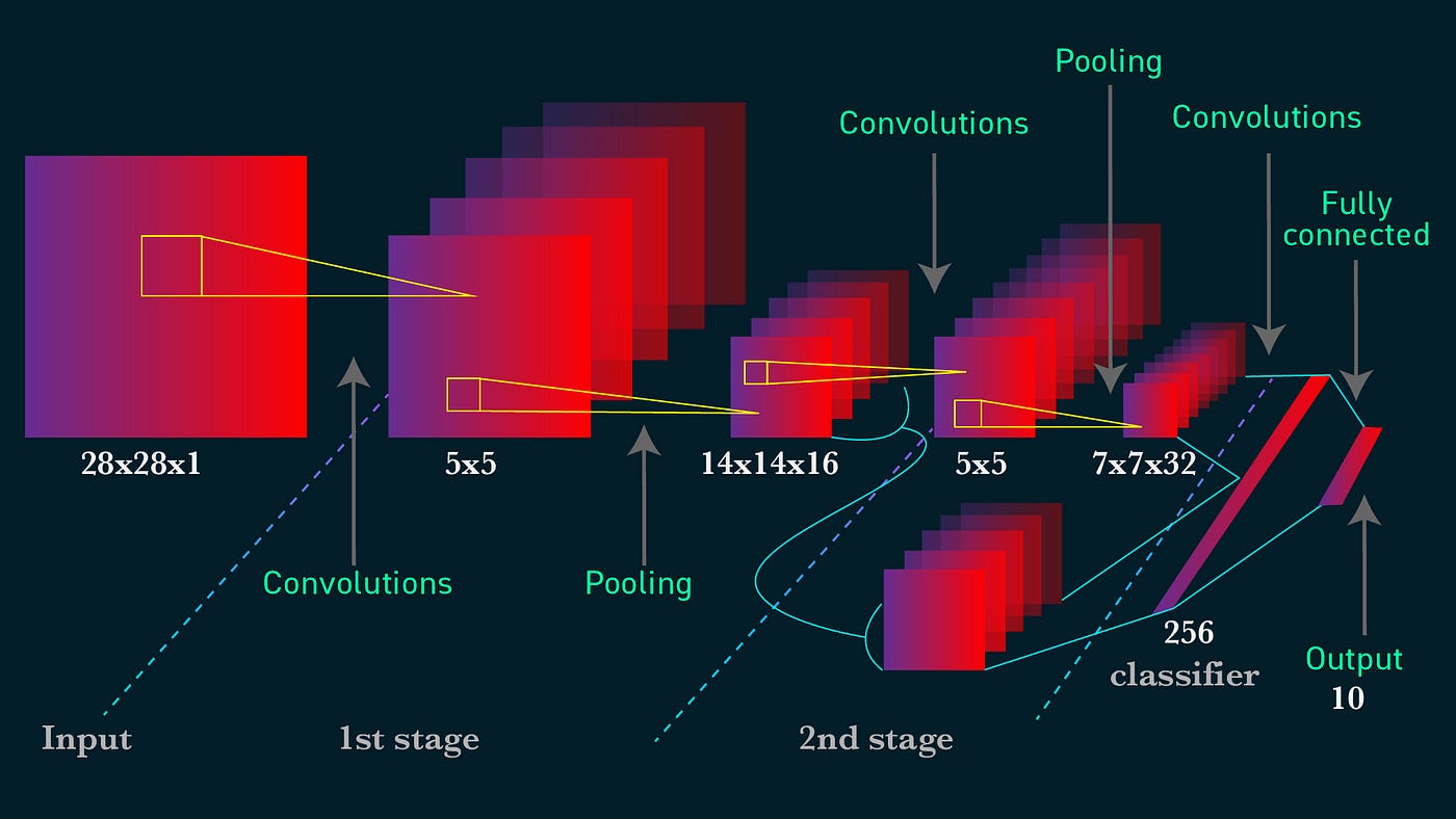
Convolutional Neural Networks (CNNs) are designed to process and analyze visual data in a hierarchical and automated manner. They consist of multiple interconnected layers that work together to extract and learn relevant features from the input image. Let’s take a closer look at how CNNs work:
1. Convolutional Layer: The first layer in a CNN is the convolutional layer. It applies a set of learnable filters, also known as convolutional kernels, to the input image. Each filter performs element-wise multiplication between its weights and a small region of the input image, known as the receptive field. This process generates feature maps that highlight important visual patterns, such as edges, textures, and shapes.
2. Activation Function: After the convolution operation, an activation function is applied element-wise to the feature maps. This introduces non-linearity and helps the network model complex relationships between the input and output. Common activation functions used in CNNs include ReLU (Rectified Linear Unit), sigmoid, and tanh.
3. Pooling Layer: The pooling layer downsamples the feature maps generated by the convolutional layer, reducing their spatial size while retaining important information. It helps make the network more efficient and robust to small variations in the input. Popular pooling techniques include max pooling and average pooling, where the maximum or average value in each pooling region is selected.
4. Fully Connected Layer: Following the convolutional and pooling layers, the fully connected layer takes the flattened output and connects every neuron to every neuron in the subsequent layer. This layer is responsible for making the final predictions or classifications based on the extracted features. The output of the fully connected layer is usually fed into a softmax function for classification tasks.
5. Backpropagation and Training: CNNs are trained using the backpropagation algorithm, where the network iteratively updates the weights and biases of its neurons to minimize a predefined loss function. This training process involves feeding the network with labeled training data, computing the loss between the predicted and actual outputs, and adjusting the parameters through gradient descent. The training continues for multiple epochs until the network achieves satisfactory performance.
6. Feature Learning: One of the standout features of CNNs is their ability to automatically learn relevant features directly from the data. Through successive convolutional and pooling layers, the network learns to recognize increasingly complex and abstract visual patterns. This hierarchical feature learning allows CNNs to excel at tasks such as image classification, object detection, and semantic segmentation.
Components of a CNN
A Convolutional Neural Network (CNN) is composed of several key components that work together to process and analyze visual data. Understanding these components is crucial for comprehending the inner workings of a CNN. Let’s explore the different components of a CNN:
1. Convolutional Layers: Convolutional layers are the backbone of a CNN. They perform the essential task of applying filters to the input data. Each filter consists of learnable weights that are convolved with small local regions of the input image, generating feature maps. These feature maps represent the learned features, such as edges, textures, and shapes.
2. Pooling Layers: Pooling layers are used to downsample the feature maps produced by the convolutional layers. They help reduce the spatial size of the feature maps while preserving the essential information. Pooling can be done using techniques such as max pooling or average pooling, where the maximum or average value in each pooling region is selected.
3. Fully Connected Layers: Fully connected layers are typically placed at the end of a CNN. They connect every neuron in one layer to every neuron in the subsequent layer. These layers are responsible for generating the final output based on the extracted features. For classification tasks, a softmax activation function is commonly used to produce the probability distribution over different classes.
4. Activation Functions: Activation functions introduce non-linearity to the CNN, allowing it to model complex relationships between the input and output. Common activation functions used in CNNs include ReLU (Rectified Linear Unit), which avoids the vanishing gradient problem, and sigmoid or softmax functions for classification problems.
5. Loss Functions: The loss function measures the discrepancy between the predicted output and the true output. It provides a quantitative measure of how well the CNN is performing. Loss functions vary depending on the task at hand, such as mean squared error for regression tasks and categorical cross-entropy for multi-class classification tasks.
6. Backpropagation: Backpropagation is a critical algorithm used to train a CNN. It involves calculating the gradients of the loss function with respect to the network’s parameters, and then using these gradients to update the weights and biases through gradient descent. Backpropagation enables the network to learn from the labeled training data and improve its performance over time.
7. Regularization Techniques: Regularization techniques, such as dropout and weight decay, are often applied in CNNs to prevent overfitting. Overfitting occurs when the network performs well on the training data but poorly on unseen data. Regularization helps to generalize the learned features and improve the CNN’s ability to make accurate predictions on new data.
8. Optimization Algorithms: Optimization algorithms, such as stochastic gradient descent (SGD), Adam, or RMSprop, are used to iteratively update the network’s parameters during the training process. These algorithms adjust the weights and biases to minimize the loss function and improve the CNN’s performance.
By combining these components, CNNs can effectively learn and extract meaningful features from visual data, making them powerful tools for tasks such as image recognition, object detection, and image generation.
Convolutional Layer
The convolutional layer is a fundamental component of a Convolutional Neural Network (CNN). It plays a crucial role in extracting and learning important features from the input data. The key idea behind the convolutional layer is to apply filters or kernels to the input image, performing convolutions to obtain feature maps.
Convolution Operation: In the convolutional layer, each filter is convolved with small receptive fields of the input image. The receptive field is a region defined by the size of the filter. The filter is then applied to all possible receptive fields to produce feature maps. The convolution process involves performing element-wise multiplications on the filter weights and the corresponding pixel values in the receptive field, followed by summing all the results.
Learnable Weights: The filters in the convolutional layer have learnable weights. During the training process, the network adjusts these weights using backpropagation and gradient descent to minimize the loss function. This allows the filters to learn patterns and extract meaningful features from the input data. For example, in an image classification task, the filters may learn to detect edges, corners, or textures.
Multiple Filters: A convolutional layer typically consists of multiple filters. Each filter learns different features, capturing a specific aspect of the input data. As a result, the convolutional layer generates multiple feature maps, each representing a different learned feature. These feature maps collectively form the output of the convolutional layer and serve as input for subsequent layers.
Stride and Padding: The stride determines the interval at which the receptive field slides across the input image. A stride of 1 means the receptive field moves one pixel at a time, while a stride of 2 moves it two pixels at a time. Strides are important for controlling the size of the output feature map. Padding, on the other hand, involves adding extra pixels around the input image to preserve the spatial size of the feature map.
Feature Hierarchy: The convolutional layer contributes to the hierarchical feature learning of CNNs. Lower layers learn low-level features, such as edges and textures, while deeper layers learn more abstract and complex features. By stacking multiple convolutional layers, CNNs can capture increasingly higher-level features, leading to a hierarchical representation of the input data.
Shared Weights: One advantage of the convolutional layer is weight sharing. Since each filter is applied to the entire input image, the same set of weights is used across the image. This reduces the number of parameters in the network and allows the CNN to capture translation-invariant features. Weight sharing contributes to the efficiency and generalization of the CNN.
Overall, the convolutional layer is a crucial building block of CNNs. It enables the network to extract informative features from the input data in a hierarchical manner, making CNNs highly effective in various computer vision tasks such as image classification, object detection, and image segmentation.
Pooling Layer
The pooling layer is an essential component of Convolutional Neural Networks (CNNs) used in computer vision tasks. It plays a key role in downsampling the feature maps produced by the convolutional layers, reducing the spatial dimensions and preserving important information. The pooling layer helps to enhance the efficiency, robustness, and translational invariance of the network.
Downsampling: The main purpose of the pooling layer is to reduce the spatial size of the feature maps while retaining relevant information. By downsampling, the pooling layer reduces the computational complexity of the network and decreases the number of parameters, making it more efficient to train and apply the CNN to large-scale datasets.
Pooling Techniques: The pooling layer performs downsampling using different pooling techniques, such as max pooling and average pooling. In max pooling, the maximum value within each pooling region is selected, representing the most prominent feature in that region. Average pooling, on the other hand, calculates the average value within each pooling region. These pooling operations effectively summarize the information in the feature maps.
Pooling Regions: The pooling layer divides the feature maps into non-overlapping or overlapping regions, known as pooling regions or pool windows. The size of the pooling regions is defined by a hyperparameter. Common choices include 2×2 or 3×3 regions with a stride of 2, which reduces the spatial dimensions by half. By choosing appropriate pooling regions, the pooling layer ensures that the downsampling is performed evenly across the feature maps.
Translational Invariance: One of the advantages of the pooling layer is its ability to introduce translational invariance to the network. Translational invariance means that the CNN can recognize certain features irrespective of their precise location in the input data. This is important for tasks like image classification, where the position of an object in an image may vary. By downsampling the feature maps, the pooling layer ensures that the network focuses on the most relevant features regardless of their spatial location.
Robustness to Variations: The pooling layer contributes to the robustness of CNNs by reducing the impact of small spatial variations in the input data. By summarizing the information in the pooling regions, the pooling layer makes the network less sensitive to minor variations, such as slight changes in the position or orientation of an object in an image. This enhances the robustness of the CNN to noise, deformations, and other distortions in the input data.
Feature Dimension: The pooling layer reduces the dimension of the feature maps by downsampling, resulting in a compressed representation of the input. This can help enhance the generalization capabilities of the network, preventing overfitting and improving the CNN’s ability to generalize well to unseen data.
Fully Connected Layer
The fully connected layer, also known as the dense layer, is a significant component of Convolutional Neural Networks (CNNs). It typically resides at the end of the network and is responsible for generating the final output based on the features learned from the preceding layers.
Connectivity: In a fully connected layer, each neuron is connected to every neuron in the previous layer. This means that every neuron receives input from all the neurons in the previous layer and sends its output to all the neurons in the following layer. This complete connectivity allows the network to make predictions or classifications based on the features extracted from the input data.
Flattening: Before the fully connected layer, the feature maps from the previous layers need to be flattened into a one-dimensional vector. This is done to meet the expectations of the fully connected layer, which accepts inputs in the form of a vector rather than a spatially organized structure. Flattening the feature maps condenses the extracted features into a manageable format for further processing.
Weight Matrix: Each connection between neurons in the fully connected layer is assigned a learnable weight. These weights parameterize the relationship between the input and the output of the fully connected layer. During the training process, these weights are adjusted through backpropagation to minimize the loss and improve the network’s performance.
Activation Function: Activation functions are applied to the outputs of the neurons in the fully connected layer to introduce non-linearity into the network. Common activation functions include ReLU (Rectified Linear Unit), sigmoid, and softmax. Activation functions allow the network to model complex relationships between the input and the output, enabling the CNN to make more sophisticated predictions.
Role in Classification: In classification tasks, the fully connected layer takes the flattened feature vectors as input and produces a probability distribution over different classes. This is typically achieved using a softmax activation function, which ensures that the outputs are normalized and sum up to 1. The class with the highest probability is taken as the predicted class label.
Feature Fusion: The fully connected layer serves as a central hub for integrating the learned features from the earlier layers. By connecting every neuron to every neuron in the subsequent layer, the fully connected layer combines the extracted information from various parts of the image to make a final decision. This feature fusion process allows the CNN to capture more global and context-aware representations.
Model Complexity: The fully connected layer contributes to the overall complexity of the CNN model. The number of neurons in the fully connected layer determines the capacity of the model to learn intricate representations. However, increasing the size of the fully connected layer also increases the number of parameters, which can lead to overfitting if not properly regulated.
The fully connected layer plays a critical role in generating the final output of a CNN. By connecting each neuron to every neuron in the previous and subsequent layers, it enables the network to recognize complex patterns and make accurate predictions based on the extracted features.
Activation Function
An activation function is a crucial component of neural networks, including Convolutional Neural Networks (CNNs). It introduces non-linearity to the network, enabling it to model complex relationships and make accurate predictions. The activation function acts on the output of each neuron in a layer, transforming it before passing it to the next layer.
Non-Linearity: One of the main reasons activation functions are used in neural networks is to introduce non-linearity. Linear functions do not have the capacity to model complex relationships between input and output. By applying non-linear activation functions, neural networks can learn and represent more intricate patterns and make non-linear predictions.
Rectified Linear Unit (ReLU): ReLU is one of the most widely used activation functions in CNNs. It sets all negative values to zero and keeps positive values unchanged. ReLU is computationally efficient, helps alleviate the vanishing gradient problem, and allows the network to learn sparse and robust representations.
Sigmoid: The sigmoid activation function squeezes the output of each neuron into the range of 0 to 1. It is often used in binary classification problems, where the network needs to output a probability between 0 and 1 for each class. However, the sigmoid function may suffer from the vanishing gradient problem and is not suitable for deep networks.
Hyperbolic Tangent (tanh): The hyperbolic tangent function is similar to the sigmoid function but maps the output to the range of -1 to 1. Tanh functions symmetrically with respect to the origin and can handle negative inputs better than the sigmoid function. Like the sigmoid function, it is susceptible to the vanishing gradient problem.
Softmax: The softmax function is commonly used in the output layer of a network for multi-class classification. It outputs a probability distribution over different classes. The softmax function normalizes the outputs, ensuring that they sum up to 1. This facilitates the interpretation of the network’s output as class probabilities.
Role in CNNs: Activation functions enable CNNs to model complex relationships between the extracted features and the target output. By introducing non-linearity, activation functions transform the linear combinations of the neuron’s inputs into more expressive representations. This allows CNNs to learn and recognize intricate patterns, enhancing their ability to tackle challenging computer vision tasks.
Choosing the Right Activation Function: The choice of activation function depends on the specific task and network architecture. ReLU is a popular choice due to its simplicity and efficiency. However, other activation functions like sigmoid and tanh may still be relevant in certain scenarios. Additionally, advanced activation functions like Leaky ReLU, Parametric ReLU, and ELU have been developed to address some of the limitations of traditional activation functions.
The activation function is a critical element in CNNs, providing non-linearity and enabling the network to learn and represent complex patterns. Choosing the appropriate activation function is crucial for achieving accurate and efficient performance in neural network applications.
Loss Function
A loss function is an essential component of training Convolutional Neural Networks (CNNs). It quantifies the discrepancy between the predicted output of the network and the true output, providing a measure of the model’s performance. The loss function guides the training process, helping the network to adjust its parameters to minimize the error and improve its predictions.
Regression Loss Functions: In regression tasks, where the goal is to predict continuous values, common loss functions include mean squared error (MSE) and mean absolute error (MAE). MSE calculates the average squared difference between the predicted and true values, while MAE calculates the average absolute difference. These loss functions evaluate the overall performance of the network and provide a measure of how well the model fits the training data.
Classification Loss Functions: In classification tasks, where the goal is to predict categorical labels, different loss functions are used. For binary classification, the binary cross-entropy loss is often employed. It calculates the average logarithmic loss between the predicted probability and the true label. For multiclass classification, the categorical cross-entropy loss is commonly used, which measures the average logarithmic loss over all classes.
Custom Loss Functions: In certain scenarios, custom loss functions may be necessary to address specific requirements of the task. For example, in object detection tasks, where both classification and localization are involved, a combination of classification loss and regression loss can be used. Additionally, loss functions like hinge loss and dice loss have been developed to tackle specific challenges in certain domains, such as image segmentation.
Gradient Descent: The loss function plays a crucial role in the optimization process during training. By calculating the gradients of the loss function with respect to the network’s parameters, the backpropagation algorithm determines how the parameters should be adjusted to minimize the loss. The optimization algorithm, such as stochastic gradient descent (SGD), uses these gradients to update the parameters iteratively, gradually improving the model’s performance.
Balance and Regularization: The choice of loss function can impact the training process and the network’s behavior. It is important to select an appropriate loss function that aligns with the specific task requirements and dataset characteristics. Additionally, regularization techniques, such as L1 and L2 regularization, can be incorporated into the loss function to avoid overfitting and encourage simpler and more generalized models.
Evaluation Metric: While the loss function is used for training, it may not always be the most meaningful metric for evaluating the performance of a model. For instance, in image classification, accuracy is a commonly used evaluation metric. It measures the proportion of correct predictions. It is crucial to consider the evaluation metric alongside the loss function to comprehensively assess the model’s effectiveness.
Backpropagation
Backpropagation is a critical algorithm used to train Convolutional Neural Networks (CNNs). It allows the network to adjust its parameters through gradient descent, iteratively optimizing the model’s performance. By calculating gradients of the loss function with respect to the network’s parameters, backpropagation guides the updates of the weights and biases, enabling the CNN to learn from labeled training data.
Forward Pass: The backpropagation algorithm starts with the forward pass, where input data is fed through the network, and predictions are generated. During the forward pass, the activations and outputs of each layer are computed sequentially, leading to the final output of the network. The forward pass involves propagating the input data through the layers, applying weight matrix multiplications and activation functions as required.
Loss Calculation: After the forward pass, the loss between the predicted output and the true output is calculated using a loss function appropriate for the task. This loss function quantifies the error in the network’s predictions, providing feedback on how well the model is performing.
Backward Pass: The backward pass, or backpropagation proper, occurs after the loss calculation. It involves calculating the gradients of the loss function with respect to the network’s parameters. Starting from the output layer, the partial derivatives, or gradients, are calculated layer by layer, propagating backward through the network.
Chain Rule: The chain rule is essential to compute the gradients during backpropagation. It allows the gradients to be calculated layer by layer by multiplying the gradients from the subsequent layer with the local gradients in each layer. This way, the gradients are efficiently propagated backward, capturing the contribution of each layer to the overall loss.
Weight and Bias Updates: After the gradients have been calculated, the optimization algorithm (e.g., stochastic gradient descent) uses these gradients to update the weights and biases of the network. The updates are made by taking small steps in the opposite direction of the gradients, aiming to minimize the loss. The step size, known as the learning rate, determines the magnitude of the weight and bias updates.
Iterations and Convergence: The backpropagation algorithm iteratively performs forward and backward passes on batches or subsets of training data. Each iteration enables the network to adjust its parameters incrementally, gradually reducing the loss and improving its predictions. The training process continues for multiple epochs until the network converges or reaches a predefined stopping criterion.
Efficiency and Regularization: Backpropagation is computationally efficient because it leverages the chain rule to calculate gradients efficiently layer by layer. To prevent overfitting and improve generalization, regularization techniques such as L1 or L2 regularization can be incorporated into the loss function during backpropagation.
Overall, backpropagation is a cornerstone of deep learning and enables Convolutional Neural Networks to learn complex patterns from input data. By iteratively adjusting the network’s parameters based on gradients calculated during the backward pass, backpropagation facilitates the optimization of CNNs and empowers them to make accurate predictions in a variety of tasks.
Training a CNN
Training a Convolutional Neural Network (CNN) involves iteratively adjusting its parameters to minimize the error and improve its performance on a specific task. The training process ensures that the CNN learns meaningful features from the input data and makes accurate predictions. Let’s explore the steps involved in training a CNN:
1. Data Preparation: The first step in training a CNN is to prepare the training data. This includes organizing the data into appropriate formats, such as image batches or feature vectors, and splitting it into training and validation sets. It is important to have a diverse and representative dataset that covers a wide range of possible inputs and outcomes.
2. Forward Pass: During the forward pass, the training data is propagated through the CNN. The input data is fed into the network, layer by layer, and activations are computed sequentially. The forward pass applies weight matrix multiplications and activation functions to transform the input into predicted outputs.
3. Loss Calculation: After the forward pass, the loss function is used to calculate the discrepancy between the predicted output and the true output. This quantifies the error of the CNN’s predictions. The objective is to minimize the loss, which indicates how well the network is fitting the training data.
4. Backpropagation and Gradient Descent: The backpropagation algorithm is utilized to calculate gradients of the loss function with respect to the network’s parameters. Starting from the output layer, these gradients are propagated backward through the network. The optimization algorithm, such as stochastic gradient descent (SGD), uses these gradients to update the weights and biases, gradually minimizing the loss and improving the network’s predictions.
5. Mini-Batch Training: To increase training efficiency and generalize well, mini-batch training is often employed. Training data is divided into smaller batches, and the forward pass and backpropagation are applied batch by batch. This allows the network to process and learn from a subset of the data at a time, leading to faster convergence and utilization of computational resources.
6. Hyperparameter Tuning: Training a CNN involves tuning various hyperparameters to achieve optimal performance. These hyperparameters include learning rate, batch size, number of layers, filter sizes, and activation functions. Finding the right combination of hyperparameters often requires experimentation and iterative adjustments to maximize the accuracy and convergence speed of the network.
7. Regularization Techniques: To prevent overfitting and improve generalization, regularization techniques are applied during training. Common techniques include dropout, which randomly deactivates neurons during training, and weight decay, which adds a penalty term to the loss function to discourage large weight values. Regularization helps the network generalize well to unseen data and perform better on test datasets.
8. Evaluation and Validation: Throughout the training process, the performance of the CNN is evaluated on a validation dataset. Metrics such as accuracy, precision, recall, and F1 score are computed to assess the model’s performance. This allows for monitoring the progress of training and making decisions regarding the learning dynamics and convergence.
9. Iterative Refinement: Training a CNN is an iterative process. The network’s parameters are updated through multiple epochs, with each epoch consisting of a complete pass through the training dataset. Through these iterations, the CNN learns and fine-tunes its parameters, gradually improving its performance and minimizing the loss on the training data.
By following these steps, training a CNN enables the network to learn from the data and adapt its parameters to make accurate predictions. It is an iterative and ongoing process that allows the network to continuously improve its performance on the target task.
Applications of CNNs
The applications of Convolutional Neural Networks (CNNs) span across various fields, revolutionizing the way we process and analyze visual data. With their ability to automatically learn and extract features, CNNs have had a substantial impact on numerous industries and domains. Let’s explore some of the key applications of CNNs:
Image Classification: CNNs excel in image classification tasks, where they can accurately categorize images into predefined classes. This has led to advancements in areas such as object recognition, facial recognition, and scene understanding. CNNs have achieved near-human performance on benchmark image classification datasets.
Object Detection: CNN-based object detection systems can identify and localize multiple objects within images or videos. These systems have immense value in fields such as autonomous driving, surveillance, and robotics, enabling real-time detection of objects and actions.
Semantic Segmentation: CNNs have made significant contributions to semantic segmentation tasks, where the goal is to assign pixel-level labels to each image region. By segmenting images into meaningful parts, CNNs facilitate tasks such as autonomous driving, medical imaging, and video understanding.
Medical Imaging: CNNs have revolutionized medical imaging analysis, aiding in tasks such as disease diagnosis, tumor detection, and lesion classification. By leveraging large-scale medical datasets, CNNs can assist radiologists and healthcare professionals in improving diagnostic accuracy and efficiency.
Natural Language Processing (NLP): Although primarily used for computer vision, CNNs have also found applications in NLP tasks. They can analyze text data, perform sentiment analysis, text classification, and even generate new text. CNNs, when combined with recurrent neural networks, have shown promising results in language translation, summarization, and question-answering tasks.
Art and Creativity: CNNs have been used to generate new and innovative art by learning patterns and styles from existing artwork. This has given rise to applications in creative fields, such as generating realistic images, transforming images using artistic styles, and creating deepfake videos.
Video Analysis: CNNs can analyze and understand videos, enabling applications such as video summarization, action recognition, and video captioning. This has opened doors for applications in video surveillance, video search, and content creation.
Agriculture and Environmental Monitoring: CNNs have been applied to remotely sensed data for crop classification, yield prediction, and environmental monitoring. This can help optimize agricultural practices, monitor deforestation, and support climate change research.
Robotics and Autonomous Systems: CNNs have played a critical role in the advancement of robotics and autonomous systems. They enable robots to perceive their surroundings, navigate environments, and interact with objects. CNN-based systems have been deployed for tasks such as robot vision, robotic grasping, and autonomous navigation.
These are just a few examples of the diverse applications of CNNs. As the field continues to evolve, CNNs are expected to further impact industries, improve efficiency, and enable new breakthroughs in areas such as healthcare, transportation, entertainment, and beyond.
Advantages of CNNs
Convolutional Neural Networks (CNNs) offer several advantages that make them highly effective in processing and analyzing visual data. Their unique architecture and design enable them to excel in various applications. Let’s explore some of the key advantages of CNNs:
Effective Feature Learning: CNNs have an innate ability to learn hierarchical representations from raw data. Through multiple layers of convolutional and pooling operations, CNNs automatically learn relevant features, such as edges, textures, and shapes, from the input data. This hierarchical feature learning allows CNNs to capture complex patterns and representations that are crucial for tasks like image classification and object detection.
Translation Invariance: CNNs are inherently translation invariant, meaning they can recognize objects regardless of their position in the input. This is achieved by applying convolutional filters to local receptive fields, allowing the network to capture local patterns and spatial dependencies. As a result, CNNs can identify objects and features even if they are shifted or rotated.
Parameter Sharing: CNNs leverage parameter sharing, which considerably reduces the number of parameters compared to fully connected networks. By using the same set of weights across different spatial locations, CNNs effectively exploit spatial locality, capturing local patterns and reducing the risk of overfitting. Parameter sharing also enables efficient computation and faster training, making CNNs more scalable and applicable to large-scale datasets.
Efficient Memory Usage: CNNs have a layered architecture that allows them to process data in a hierarchical manner. This reduces the memory requirement as only a subset of the network is active at a given time. By reusing feature maps and learning from local patterns, CNNs optimize memory usage, enabling them to handle large images and videos efficiently.
Robustness to Variations: CNNs are robust to variations in the input, such as changes in lighting, scale, and orientation. This is because CNNs can learn generalizable representations from augmented and diverse training data. The hierarchical feature learning also helps the network focus on the most relevant and discriminative features, making CNNs robust to noise and variations in the input data.
Parallel Processing: CNNs are highly amenable to parallel processing, making them suitable for implementation on modern parallel computing architecture, such as GPUs. The convolutional and pooling operations can be performed simultaneously on different regions of the input, accelerating the computations and enabling real-time applications.
State-of-the-Art Performance: CNNs have consistently achieved top performance on benchmark datasets and tasks, surpassing previous methods in computer vision and deep learning. CNNs have become the de facto standard for image classification, object detection, and semantic segmentation, setting new benchmarks and pushing the boundaries of what is achievable in visual analysis tasks.
Together, these advantages make CNNs a powerful tool for processing visual data. Their ability to learn hierarchical representations, handle translations and variations, and leverage parallel processing has propelled CNNs to be the go-to architecture for many computer vision tasks, empowering breakthroughs across numerous domains.
Limitations of CNNs
While Convolutional Neural Networks (CNNs) excel in many applications, there are certain limitations to be aware of when using this architecture for processing and analyzing visual data:
Limited Spatial Context: CNNs have a limited spatial context due to the use of small receptive fields in the convolutional layers. This means that CNNs may not fully capture long-range dependencies and context information that could be important for certain tasks. This limitation can be mitigated by incorporating larger receptive fields or by utilizing more advanced architectures.
Large Training Data Requirements: CNNs typically require a large amount of labeled training data to learn effective representations. Collecting and annotating large datasets can be resource-intensive, especially for specialized domains or tasks. Limited data availability can impact the performance and generalization ability of CNNs, potentially leading to overfitting.
Computational Complexity: Training CNNs, especially deeper and more complex architectures, can be computationally intensive and time-consuming. The large number of parameters and the nature of convolutions result in substantial memory and processing requirements. Employing CNNs on resource-limited devices or in real-time applications can be a challenge, requiring optimization strategies and alternative architectures.
Lack of Interpretable Representations: CNNs are often considered as black box models due to their complex internal representations. Understanding exactly how and why CNNs make predictions can be difficult. Extracting human-interpretable features and explanations from CNNs remains an ongoing research area, hindering their interpretability and explainability.
Difficulty Handling Variations: While CNNs are generally robust to certain variations in the input, they may struggle with handling extreme variations or novel examples outside the training distribution. Fine-tuning or retraining on new data is often necessary to adapt CNNs to different domains or scenarios. Additionally, adversarial attacks can exploit vulnerabilities in CNNs by introducing imperceptible perturbations to the input, resulting in misclassifications.
Domain-Specific Knowledge: CNNs are not born with prior domain knowledge; they need to learn from the available data. This means that CNNs may struggle in tasks where prior knowledge or specialized domain information is essential. Incorporating domain-specific knowledge or leveraging transfer learning from pre-trained models can help mitigate this limitation.
Limited Recurrent Information: CNNs primarily leverage feed-forward operations, which may limit their ability to process sequential or temporal data. Tasks that require contextual understanding across time or long-range dependencies may not be well-suited for standard CNN architectures. Recurrent Neural Networks (RNNs) or their variants, such as Long Short-Term Memory (LSTM) networks, are often more suitable for such tasks.
Understanding and addressing these limitations are crucial when working with CNNs. Overcoming these challenges involves ongoing research and engineering efforts to improve the model architecture, training techniques, interpretability, and generalizability of CNNs for a wide range of applications.