How to Strikethrough In Excel

Why Strikethrough Is Useful in Excel

Strikethrough is a valuable formatting option in Excel that allows you to visually denote changes or indicate completed or canceled items. It is particularly useful in various scenarios, such as:

Tracking Changes: When collaborating on a spreadsheet with multiple team members, using strikethrough can easily highlight modifications made to specific cells. You can quickly identify what data has been updated, providing a clear visual cue without the need for extensive explanations.
Managing To-Do Lists: Strikethrough is ideal for managing to-do lists or task trackers in Excel. When a task is completed, you can strike through the respective cell to indicate its status. This simple formatting technique saves time and reduces ambiguity, ensuring that everyone knows what tasks are still pending.
Cancelling Data: Strikethrough is great for canceling out information that is no longer valid or relevant. Whether it’s a price change, an outdated formula, or an incorrect entry, applying a strikethrough to such cells immediately communicates that the data should no longer be considered.
Highlighting Discrepancies: Strikethrough can be used to mark inconsistencies in data or identify potential errors. For example, when comparing two sets of numbers, you can apply strikethrough to the cells with lower values to draw attention to the discrepancies.

By leveraging the strikethrough feature in Excel, you can enhance the clarity and readability of your spreadsheets, streamlining data management and improving collaboration among team members. It serves as a helpful indicator, allowing you to visually convey changes and make your data easier to understand at a glance.

How to Apply Strikethrough to Selected Cells

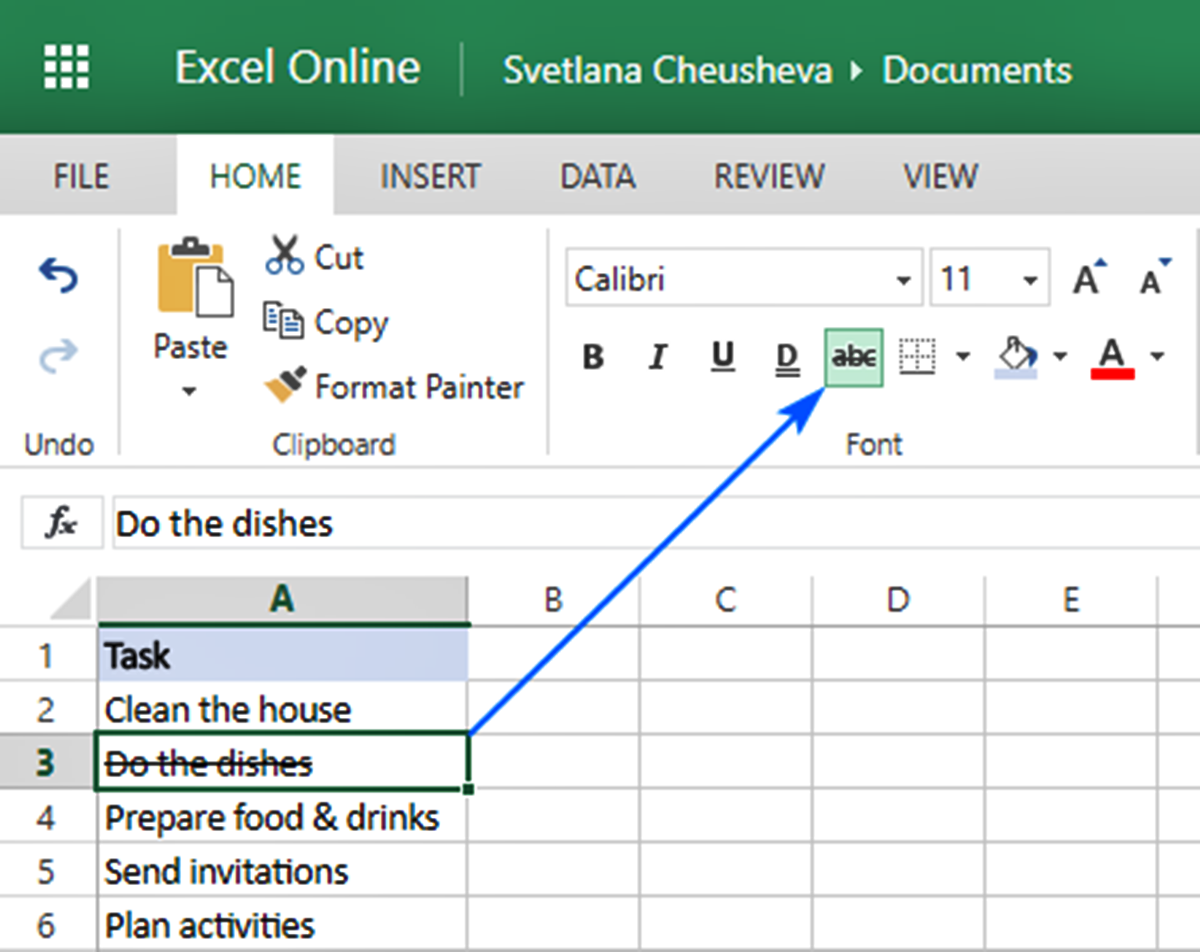
Applying strikethrough formatting to selected cells in Excel is a straightforward process. Here’s how you can do it:

Select the cells or range of cells that you want to apply strikethrough to. To select multiple non-adjacent cells, hold down the Ctrl key while selecting the desired cells.
Right-click on the selected cells and choose “Format Cells” from the context menu. Alternatively, you can go to the “Home” tab in the Excel ribbon and click on the “Format Cells” button in the “Font” group.
In the “Format Cells” dialog box, switch to the “Font” tab.
Check the “Strikethrough” checkbox in the “Effects” section to apply strikethrough to the selected cells.
Click “OK” to save the changes and close the dialog box.

Once you follow these steps, the selected cells will be formatted with strikethrough, making it easy to visually differentiate them from other cells in the spreadsheet.

It’s important to note that applying strikethrough in this manner is a manual process. If you need to update the cell contents or modify the data, you will need to reapply the strikethrough formatting if necessary.

Additionally, you can also utilize shortcuts to apply strikethrough formatting more efficiently. By selecting the cells and pressing the combination of “Ctrl” + “5,” you can quickly apply strikethrough to the selected cells without opening the “Format Cells” dialog box.

Remember, strikethrough is just one of many formatting options available in Excel. It can greatly enhance the visual clarity of your spreadsheets, enabling you to effectively communicate changes or indicate completed tasks.

How to Remove Strikethrough from Cells

Removing strikethrough formatting from cells in Excel is a simple process. Here are the steps to remove the strikethrough from selected cells:

Select the cells or range of cells from which you want to remove the strikethrough. You can select multiple non-adjacent cells by holding down the Ctrl key while selecting the desired cells.
Right-click on the selected cells and choose “Format Cells” from the context menu. Alternatively, you can go to the “Home” tab in the Excel ribbon and click on the “Format Cells” button in the “Font” group.
In the “Format Cells” dialog box, switch to the “Font” tab.
Uncheck the “Strikethrough” checkbox in the “Effects” section to remove the strikethrough from the selected cells.
Click “OK” to save the changes and close the dialog box.

By following these steps, you can easily remove the strikethrough formatting from the selected cells, restoring them to their original appearance.

Alternatively, if you want to remove strikethrough from individual cells or a few selected cells without accessing the “Format Cells” dialog box, you can use the following keyboard shortcut: press “Ctrl” + “5” while the cells are selected. This shortcut toggles the strikethrough formatting on and off.

Keep in mind that if you have applied strikethrough formatting using conditional formatting rules or formulas, you will need to modify or remove those rules to completely remove the strikethrough effect.

Removing strikethrough formatting allows you to update the cell contents or modify the data without the visual indicator of a strikethrough. It is especially useful when managing dynamic data or when the need for the formatting no longer applies.

Remember to carefully confirm that you have removed the strikethrough for the intended cells to avoid any confusion or misinterpretation of the data in your Excel spreadsheet.

Using Keyboard Shortcuts for Strikethrough

Excel offers convenient keyboard shortcuts that allow you to quickly apply and remove strikethrough formatting without navigating through multiple menus. Knowing these shortcuts can significantly improve your productivity. Here are some commonly used keyboard shortcuts for applying and removing strikethrough:

Apply Strikethrough: Select the cells you want to apply strikethrough to, then press Ctrl + 5. This shortcut instantly applies strikethrough formatting to the selected cells.
Remove Strikethrough: To remove strikethrough from cells, select the cells with strikethrough formatting and press Ctrl + 5 again. The shortcut toggles the strikethrough effect on and off, allowing you to easily remove the formatting.

By making use of these keyboard shortcuts, you can save valuable time and make your strikethrough workflow more efficient. Instead of navigating through menus and dialog boxes, you can apply or remove strikethrough with just a few simple keystrokes.

It’s important to note that these keyboard shortcuts work for both individual cells and ranges of cells. You can select multiple non-adjacent cells by holding down the Ctrl key while selecting each cell.

Additionally, you can combine the strikethrough shortcut with other formatting shortcuts to further enhance your Excel experience. For example, you can use Ctrl + B to apply bold and strikethrough formatting simultaneously or Ctrl + U to apply underline and strikethrough formatting together.

Mastering keyboard shortcuts can significantly improve your efficiency when working with Excel. Take the time to practice and memorize these shortcuts to streamline your workflow and become a more proficient Excel user.

Applying Strikethrough to Conditional Formatting

Conditional formatting in Excel allows you to dynamically apply formatting to cells based on specific conditions or criteria. By combining conditional formatting with strikethrough, you can create powerful visual cues and highlight specific data points in your spreadsheet. Here’s how you can apply strikethrough to conditional formatting:

Select the range of cells you want to apply the conditional formatting to. This can be a single column, a row, or a range of cells.
Go to the “Home” tab in the Excel ribbon and click on the “Conditional Formatting” button in the “Styles” group. From the dropdown menu, select “New Rule.”
In the “New Formatting Rule” dialog box, choose the option “Format only cells that contain” under the “Select a rule type” section.
In the “Format only cells with” dropdown, select the appropriate condition that you want to apply the strikethrough formatting to. It could be “Cell Value,” “Text,” “Dates,” or any other relevant option.
In the “Format only cells with” section, define the specific criteria for applying the formatting. For example, if you want to strikethrough cells where the value is less than 0, input the appropriate condition and value.
Click on the “Format” button to open the “Format Cells” dialog box.
In the “Font” tab of the “Format Cells” dialog box, check the “Strikethrough” checkbox under the “Effects” section.
Click “OK” to close the “Format Cells” dialog box.
Click “OK” in the “New Formatting Rule” dialog box to save the conditional formatting rule.

By following these steps, you can apply strikethrough formatting to cells that meet specific criteria defined by conditional formatting rules. This allows you to effectively highlight and differentiate data points based on their values or characteristics.

Conditional formatting with strikethrough is particularly useful for tasks such as identifying overdue tasks, tracking changes in financial data, or flagging incomplete items. It not only enhances the visual presentation of your spreadsheet but also provides valuable insights at a glance.

How to Use Conditional Formatting to Apply Strikethrough to Cells

Conditional formatting in Excel allows you to apply formatting to cells based on specific criteria or conditions. By combining conditional formatting with strikethrough, you can visually highlight and draw attention to certain cells in your spreadsheet. Here are the steps to use conditional formatting to apply strikethrough to cells:

Select the range of cells you want to apply the conditional formatting to. This can be a single column, a row, or a range of cells.
Go to the “Home” tab in the Excel ribbon and click on the “Conditional Formatting” button in the “Styles” group. From the dropdown menu, select “New Rule.”
In the “New Formatting Rule” dialog box, choose the option “Use a formula to determine which cells to format.”
In the formula field, enter the formula that defines the condition for the strikethrough formatting. For example, if you want to apply strikethrough to cells with values less than 0, you can use the formula “=A1<0" (assuming that cell A1 is the top-left cell of the selected range).
Click on the “Format” button to open the “Format Cells” dialog box.
In the “Font” tab of the “Format Cells” dialog box, check the “Strikethrough” checkbox under the “Effects” section.
Click “OK” to close the “Format Cells” dialog box.
Click “OK” in the “New Formatting Rule” dialog box to save the conditional formatting rule.

By following these steps, Excel will apply the strikethrough formatting to cells that meet the specified condition in the conditional formatting rule.

You can use a wide range of formulas and conditions to determine which cells should have the strikethrough formatting. This provides you with the flexibility to apply strikethrough based on various criteria, such as values, text contents, dates, or custom logic.

Conditional formatting with strikethrough is beneficial for tasks such as tracking milestones, identifying completed tasks, or highlighting specific data points that meet certain conditions.

Remember that you can always modify or delete the conditional formatting rule as needed. This allows you to adapt the formatting based on changes in your data or criteria.

How to Format Strikethrough Styles

When working with strikethrough in Excel, you have the option to customize the style and appearance of the strikethrough line. Here are the steps to format strikethrough styles to suit your preferences:

Select the cells or range of cells that have the strikethrough formatting applied.
Right-click on the selected cells and choose “Format Cells” from the context menu. Alternatively, you can go to the “Home” tab in the Excel ribbon and click on the “Format Cells” button in the “Font” group.
In the “Format Cells” dialog box, switch to the “Font” tab.
Click on the “Strikethrough” dropdown button to reveal a variety of strikethrough styles.
Select the desired style from the dropdown menu. Excel offers different styles, including single line, double line, words only, and more.
Preview the selected strikethrough style in the preview section of the “Format Cells” dialog box.
Adjust other formatting options, such as font style, size, and color, as desired.
Click “OK” to save the changes and apply the new strikethrough style.

By following these steps, you can easily customize the appearance of the strikethrough line to match your specific requirements or personal preferences.

In addition to the available styles, Excel also allows you to create your own custom strikethrough style. To do this, you will need to use a combination of other formatting options, such as borders or shapes. By experimenting with different formatting techniques, you can create unique and visually appealing strikethrough effects.

Remember that the strikethrough style is applied to the entire cell. If you want to apply strikethrough to only a portion of the cell’s contents, you can use a workaround by inserting a shape or textbox with the desired strikethrough style and positioning it over the text.

Keep in mind that the availability of certain strikethrough styles may vary depending on the version of Excel you are using. Some older versions may have limited options or may not support advanced strikethrough styles.

By leveraging the formatting options for strikethrough, you can enhance the visual presentation and readability of your Excel data, making it easier to communicate changes or emphasize important information.

Tips and Tricks for Working with Strikethrough in Excel

Working with strikethrough formatting in Excel can greatly improve the readability and organization of your data. Here are some tips and tricks to enhance your experience:

Combine Strikethrough with Other Formatting: Strikethrough can be combined with other formatting options, such as bold, italic, or underline. By using different combinations, you can create more visually appealing and informative formats.
Conditional Formatting with Strikethrough: Take advantage of conditional formatting to automatically apply strikethrough to cells based on specific conditions. This can help you highlight relevant data and draw attention to specific values or occurrences.
Use Shortcut Keys: Shortcut keys can save you time when applying or removing strikethrough formatting. For example, press Ctrl + 5 to apply or remove strikethrough from selected cells quickly.
Copy and Paste Formats: If you have applied strikethrough formatting to a cell and want to transfer the formatting to other cells, use the Format Painter tool. This saves time by eliminating the need to manually apply strikethrough to each cell.
Clear Formatting: If you want to remove all formatting, including strikethrough, from a cell or range of cells, select the cells and press Ctrl + Spacebar to select the entire column, or Shift + Spacebar to select the entire row. Then, press Ctrl + Shift + _ (underscore) to remove the formatting.
Modify Strikethrough Thickness: If you want to adjust the thickness of the strikethrough line, you can use VBA (Visual Basic for Applications) macros to customize the formatting. This allows you to achieve your desired visual effect.
Print Preview: Before printing your Excel spreadsheet, use the Print Preview feature to ensure that the strikethrough formatting appears as expected. This helps you identify any potential issues and make necessary adjustments.
Be Consistent: When applying strikethrough formatting, be consistent throughout your spreadsheet. Ensure that you use the same strikethrough style and color for related data points to maintain clarity and coherence.
Document Your Formatting: If you are sharing your Excel files with others, it’s a good practice to include a legend or a note explaining the significance of the strikethrough formatting. This helps others understand the meaning behind the formatting choices.

By leveraging these tips and tricks, you can work more efficiently with strikethrough formatting in Excel, improving the organization, readability, and overall effectiveness of your spreadsheets.