How Do You Alphabetize in Excel?

What is Alphabetizing in Excel?

Alphabetizing in Excel refers to the process of arranging data in a specific column or columns in alphabetical order. It is a useful feature that allows you to sort and organize data more efficiently, making it easier to find and analyze information. Whether you’re working with a list of names, titles, or any other type of data, alphabetizing can help you quickly locate specific entries and identify patterns or anomalies.

Excel provides a seamless way to alphabetize data, whether it’s a single column or multiple columns. By using the sorting functions in Excel, you can rearrange your data in ascending (A to Z) or descending (Z to A) order based on the values in the selected column(s). This feature can be particularly valuable when dealing with large datasets or when you need to present information in a more structured and organized manner.

In addition to standard alphabetizing, Excel also allows you to customize the sort order, handle special characters and numbers, remove duplicates, and undo any changes made during the sorting process. These features give you greater control and flexibility when working with your data, ensuring that it is sorted and displayed exactly how you need it.

Alphabetizing in Excel is especially beneficial in a variety of scenarios, such as:

Organizing a list of names, such as a contact list or customer database.
Arranging titles or headings in alphabetical order for a report or presentation.
Sorting product names, SKU numbers, or inventory data in a sales spreadsheet.
Grouping and categorizing data based on specific criteria, such as locations or departments.

By mastering the art of alphabetizing in Excel, you can streamline your workflow, save time, and enhance data analysis. Now that you understand the foundation of alphabetizing, let’s explore how to perform this task in Excel efficiently.

How to Alphabetize in Excel

Alphabetizing data in Excel is a straightforward process that can be completed in just a few simple steps. Whether you’re working with a single column or multiple columns, Excel provides a variety of tools to help you sort your data alphabetically.

To alphabetize a single column, follow these steps:

Select the column you want to alphabetize by clicking on the column header.
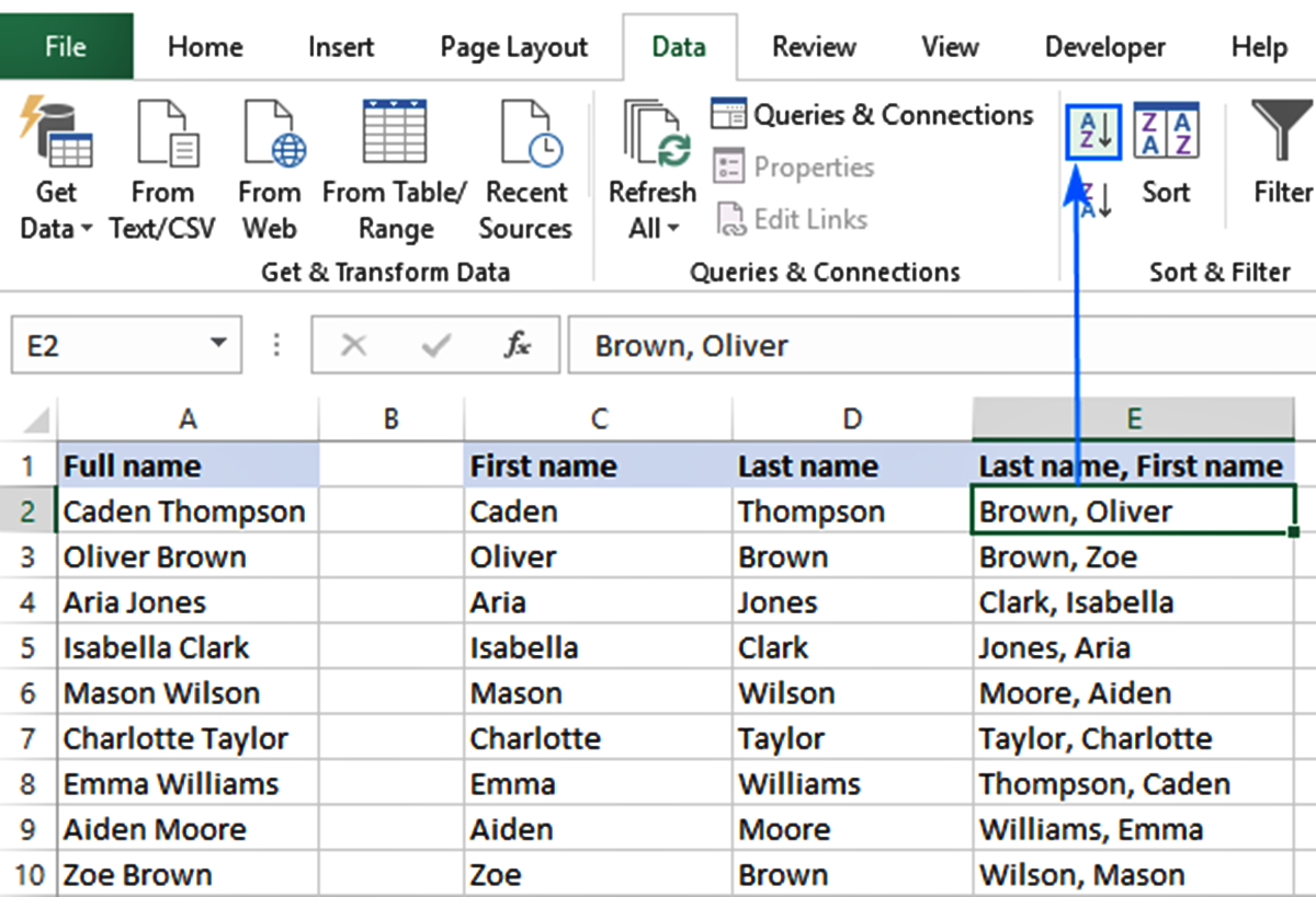
Go to the Data tab in the Excel toolbar.
Click on the Sort A to Z button to sort the column in ascending order (A to Z). If you want to sort in descending order (Z to A), click on the Sort Z to A button.

If you want to alphabetize multiple columns based on a certain column, use the following steps:

Select the range of cells that contain the data you want to sort.
Go to the Data tab in the Excel toolbar.
Click on the Sort button to open the Sort dialog box.
In the Sort dialog box, choose the column you want to sort by from the Sort by dropdown menu.
Specify the sort order as either Ascending or Descending.
Click on the OK button to apply the alphabetizing to the selected columns.

By following these steps, you can easily alphabetize your data in Excel and ensure that it is organized in a way that suits your needs. Additionally, Excel allows you to further customize the alphabetizing order and handle special characters and numbers.

Note: Remember to always save your file before making any changes, as sorting data in Excel is irreversible and will modify the original order of your data.

Now that you know how to alphabetize in Excel, you can manage your data more effectively and make it easier to locate, analyze, and present information in a clear and concise manner.

Alphabetizing a Single Column

Alphabetizing a single column in Excel is a simple process that can help you quickly organize and sort your data. Whether you have a list of names, product categories, or any other type of information, alphabetizing will make it easier for you to find specific entries or analyze the data more effectively.

To alphabetize a single column in Excel, follow these steps:

Select the column you want to alphabetize by clicking on the column header. You can do this by clicking on the letter corresponding to the column, such as ‘A’ for column A.
Once the column is selected, go to the Data tab in the Excel toolbar.
Locate the Sort section and click on the Sort A to Z button to sort the column in ascending order (A to Z). If you want to sort in descending order (Z to A), click on the Sort Z to A button.

Excel will automatically rearrange the data in the selected column based on the alphabetical order of the entries. The rest of your worksheet will remain unaffected, allowing you to maintain the integrity of your data.

If your column contains blank cells or cells with formulas, Excel will sort these cells to the top or bottom of your data, depending on your sort order. This will help ensure that your data remains well-organized and easy to navigate.

Note: It’s important to make sure that your data doesn’t contain any merged cells, as this can affect the accuracy of the sorting process. If you’re encountering any issues with alphabetizing a column, double-check for merged cells and unmerge them if necessary.

Whether you’re alphabetizing names in a contact list or categories in a product inventory, alphabetizing a single column in Excel is a valuable skill that can make your data more manageable and accessible. By following these steps, you can easily arrange your data in alphabetical order and streamline your workflow.

Alphabetizing Multiple Columns

Alphabetizing multiple columns in Excel allows you to sort and organize data across different columns based on a specific column’s values. This can be particularly useful when working with complex datasets, where you need to arrange information in a cohesive and structured manner.

Here’s how you can alphabetize multiple columns in Excel:

Select the range of cells that contain the data you want to sort. You can do this by clicking and dragging to highlight the desired cells.
Go to the Data tab in the Excel toolbar.
In the Sort section, click on the Sort button. This will open the Sort dialog box.
In the Sort dialog box, choose the column you want to sort by from the Sort by dropdown menu. This column will be the primary sorting criterion for your data.
Specify the sort order as either Ascending or Descending.
If you want to prioritize secondary sorting criteria, you can add additional levels by clicking on the Add Level button. This allows you to further refine the sorting order by selecting other columns and sort conditions.
Click on the OK button to apply the alphabetizing to the selected columns.

Excel will then rearrange the data based on the sorting criteria you specified. The primary column you selected will be the primary sorting factor, followed by any secondary sorting levels you added. This provides a comprehensive and organized view of your data across multiple columns.

When alphabetizing multiple columns, keep in mind that Excel will prioritize the primary sorting criterion and then use the subsequent levels to further refine the sorting order. This can be beneficial when you have multiple columns that need to be sorted based on specific conditions.

By mastering the skill of alphabetizing multiple columns in Excel, you can effectively manage and analyze complex datasets. It allows you to organize data in a way that best suits your needs and makes information retrieval and analysis more efficient.

Sorting Rows Based on a Specific Column

In Excel, you can sort rows based on the values in a specific column. This allows you to arrange your data in a way that focuses on the particular criteria you choose, making it easier to analyze information and identify patterns or trends.

To sort rows based on a specific column in Excel, follow these steps:

Select the range of cells that contains the data you want to sort. This can be done by clicking and dragging to highlight the desired cells.
Go to the Data tab in the Excel toolbar.
In the Sort section, click on the Sort button. This will open the Sort dialog box.
In the Sort dialog box, choose the column you want to sort by from the Sort by dropdown menu.
Specify the sort order as either Ascending or Descending.
Click on the OK button to apply the sorting to the selected range of cells.

Excel will then sort the rows based on the values in the chosen column, either in ascending (A to Z) or descending (Z to A) order. The rest of the columns in your spreadsheet will follow the sorting order of the selected column, ensuring that your data remains coherent and well-organized.

Sorting rows based on a specific column is particularly useful when you have a large dataset with multiple columns and need to focus on a particular aspect of the data. For example, if you have a sales spreadsheet with columns for product names, quantities, and prices, you can sort the rows based on the price column to identify the highest or lowest priced products.

By sorting rows based on a specific column, you can effectively analyze data and gain a deeper understanding of the information at hand. This feature allows you to tailor your view of the data to meet your specific requirements and make more informed decisions based on the sorted results.

Customizing the Alphabetizing Order

Excel provides the flexibility to customize the alphabetizing order based on your specific needs. You can adjust the default A to Z or Z to A sorting order to meet the requirements of your data. This customization allows you to sort data in a way that makes the most sense for your particular dataset.

To customize the alphabetizing order in Excel, follow these steps:

Select the column or range of cells that you want to alphabetize.
Go to the Data tab in the Excel toolbar.
In the Sort section, click on the Sort A to Z or Sort Z to A button, depending on the initial order of your data.
In the Sort Options dialog box, select the Custom List option.
Click on the Import button and choose a custom sorting order file if you have one. Custom sorting order files allow you to define a specific order for your data.
If you don’t have a custom sorting order file, you can manually customize the order by typing the desired values in the List Entries box. Separate each value with a comma.
Click on Add to add the custom entries to the sort list.
Specify the sort order as either Ascending or Descending and click on OK to apply the custom sorting order.

By customizing the alphabetizing order, you can ensure that your data is sorted in a way that aligns with your specific requirements. This can be particularly useful when dealing with datasets that have unique sorting arrangements, such as custom categories, specialized terms, or non-alphabetic symbols.

Excel also allows you to save the custom sorting order as a file, making it easy to reuse the custom list in future sorting operations.

Customizing the alphabetizing order in Excel gives you greater control over how your data is sorted and organized. It allows you to create a more tailored view of your data and enhances your ability to analyze and interpret the information effectively.

Handling Special Characters and Numbers while Alphabetizing

When alphabetizing data in Excel, you may encounter special characters and numbers that need to be sorted along with alphabetical values. Excel provides options to handle these special characters and numbers while alphabetizing, ensuring that your data is sorted in a logical and meaningful way.

Here are some techniques to handle special characters and numbers while alphabetizing in Excel:

Keeping special characters and numbers in their original position: By default, Excel will move special characters, numbers, and punctuation to the top or bottom when alphabetizing. However, if you want to keep them in their original position within the data, you can create a helper column and assign unique values to them. Then, sort the data based on the helper column along with the original column to maintain the desired order.
Ignoring special characters and numbers: If you prefer to ignore special characters and numbers while alphabetizing, you can use the built-in options in Excel. When sorting, you can choose to ignore leading spaces, case sensitivity, and punctuation. This will allow you to focus solely on the alphabetical values in the data.
Customizing sorting rules: Excel also allows you to customize the sorting rules to handle specific characters or symbols in a preferred way. You can create a custom sorting list and assign specific orders to special characters and numbers. This enables you to prioritize or group them as necessary.

By using these techniques, you can effectively handle special characters and numbers while alphabetizing your data in Excel. This ensures the accurate sorting of your data, maintaining the integrity of your information and allowing for easy analysis and interpretation.

Remember, it’s important to consider the specific needs of your dataset and the desired outcome when deciding how to handle special characters and numbers while alphabetizing. This will ensure that the resulting order aligns with your intentions and enhances the clarity and usefulness of your sorted data.

Removing Duplicates after Alphabetizing

After alphabetizing your data in Excel, you may find that there are duplicate entries within the sorted list. Duplicates can clutter your data and make it more challenging to analyze and interpret. Fortunately, Excel offers a feature that allows you to easily remove duplicates after alphabetizing, streamlining your dataset and enhancing its clarity.

To remove duplicates after alphabetizing in Excel, follow these steps:

Select the column or range of cells containing the alphabetized data.
Go to the Data tab in the Excel toolbar.
In the Data Tools section, click on the Remove Duplicates button. This will open the Remove Duplicates dialog box.
In the Remove Duplicates dialog box, choose the column(s) that contain the data you want to check for duplicates. By default, Excel selects all columns in the range you have selected.
Click on the OK button to remove the duplicate entries.

Excel will scan the selected range for duplicate entries based on the specified column(s). It will remove any duplicate values, leaving only unique entries in your dataset.

Removing duplicates is particularly useful when working with large datasets or when creating accurate reports and databases. It allows you to maintain data integrity and ensures that each entry is unique, providing a more reliable basis for analysis and decision-making.

Note: When removing duplicates, exercise caution and double-check the preview of the duplicate values before confirming the removal. This ensures that you are not unintentionally deleting any important data.

By removing duplicates after alphabetizing, you can declutter your dataset and create a more concise and accurate representation of your information. This enhances the effectiveness of your analysis and simplifies the process of extracting valuable insights from your sorted data.

Undoing Alphabetizing in Excel

While alphabetizing in Excel can be a valuable tool for organizing and analyzing data, there may be instances where you need to undo the sorting and revert your data to its original order. Whether you made a mistake during the sorting process or simply want to restore the initial arrangement, Excel provides a simple method to undo alphabetizing.

To undo alphabetizing in Excel, you can use the Undo feature or follow these steps:

Click on the cell in the column that was alphabetized.
Go to the Data tab in the Excel toolbar.
In the Sort & Filter section, click on the Sort A to Z or Sort Z to A button, depending on the previous sorting order.

By clicking the same sorting button again, Excel will revert the sorting order back to the original state, effectively undoing the alphabetizing process. This restores your data to its initial arrangement before the sorting was applied.

Note: It is important to note that the Undo feature in Excel allows you to reverse the most recent action, including alphabetizing. Simply press “Ctrl + Z” on your keyboard or click on the Undo button in the toolbar to undo the sorting instantly. However, this feature has limitations and may not be available if you have made additional changes or performed other operations after alphabetizing.

Undoing alphabetizing in Excel gives you the flexibility to correct any errors or make adjustments to your data without losing the original order. It allows you to maintain data integrity and easily modify the sort order to meet your specific needs.

Remember to save your file periodically to preserve different versions of your data, ensuring that you can revert back to any previous state if needed. This provides an extra layer of protection and allows you to navigate and manipulate your data with confidence in Excel.

Troubleshooting Common Issues with Alphabetizing

While alphabetizing data in Excel is generally a straightforward process, there are a few common issues that users may encounter. These issues can impact the accuracy and effectiveness of the sorting operation. By understanding and addressing these problems, you can ensure smooth and error-free alphabetizing in Excel.

Here are some common issues that you may encounter while alphabetizing in Excel, along with solutions to troubleshoot them:

1. Merged Cells: If your data contains merged cells, it can affect the sorting process. Excel treats merged cells as a single entity, and sorting them may not produce the desired results. To resolve this issue, unmerge any cells in the affected range before alphabetizing.

2. Hidden Rows or Columns: Hidden rows or columns can interfere with the sorting operation, causing unexpected results. Make sure to unhide any hidden rows or columns before alphabetizing to ensure accurate sorting.

3. Mixed Data Types: If your column contains a mixture of data types, such as numbers and text, Excel may encounter difficulties in determining the correct sorting order. Ensure that your data is consistent in terms of its data type to avoid any sorting errors.

4. Leading Spaces: Leading spaces in cells can impact the sorting order in Excel. It’s important to remove any leading or trailing spaces from your data before alphabetizing to ensure that the sorting is accurate. You can use the TRIM function to eliminate any leading spaces in your data.

5. Case Sensitivity: By default, Excel considers uppercase and lowercase letters as different characters when alphabetizing. If you want to ignore case sensitivity, select the “Case Sensitive” option in the Sort dialog box to ensure that the sorting order remains consistent regardless of letter case.

6. Sorting Range: Ensure that you have selected the correct range of cells for sorting. If you accidentally select a range that doesn’t include all the necessary data, the sorting may not produce the desired outcome.

7. Large Datasets: Sorting large datasets can take a significant amount of time and may result in performance issues. To improve sorting speed, consider narrowing down your range or using the “Sort” feature in smaller portions of the data.

By addressing these common issues, you can troubleshoot any problems that may arise during the alphabetizing process in Excel. This will help you achieve accurate and reliable results, ensuring that your data is sorted in a way that aligns with your intended order.