
What Is a Linear Model?
A linear model is a fundamental concept in machine learning that involves the use of a linear equation to represent the relationship between input variables and the corresponding target variable. It assumes a linear relationship between the input and output, i.e., a straight line that can be used to predict the outputs for unseen inputs. This powerful modeling technique has applications in various domains, including finance, healthcare, and marketing.
The basic idea behind a linear model is to find the best-fitting line that minimizes the distance between the predicted output and the actual output. This line is determined by estimating the coefficients or weights assigned to each input variable, which can be adjusted during the training process to improve the accuracy of predictions. The equation for a simple linear model can be written as:
y = b0 + b1x1 + b2x2 + … + bnxn
Here, y represents the target variable, x1, x2, …, xn are the input variables, and b0, b1, b2, …, bn are the coefficients assigned to each input variable. The goal is to find the optimal values for these coefficients that minimize the difference between the predicted and actual values.
Linear models are particularly useful when there is a linear relationship between the input and output variables, as they provide a simple and interpretable solution. However, it is important to note that they may not be suitable for complex and nonlinear relationships, as they have limited flexibility in capturing such patterns.
It’s worth mentioning that linear models can be implemented using different algorithms, such as ordinary least squares (OLS), ridge regression, and Lasso regression. These algorithms offer different ways to estimate the coefficients and handle specific scenarios, such as multicollinearity or overfitting.
Understanding the Basics of Linearity
Linearity is a fundamental concept in the context of linear models. It refers to the property of a relationship between input variables and the target variable that can be represented by a straight line. Understanding linearity is crucial for interpreting and building effective linear models.
In a linear relationship, the change in the target variable is directly proportional to the change in the input variables. This means that if one input variable increases by a certain amount, the target variable will increase or decrease accordingly, based on the coefficients assigned to that variable. Similarly, if multiple input variables change simultaneously, the target variable will respond in a linear fashion.
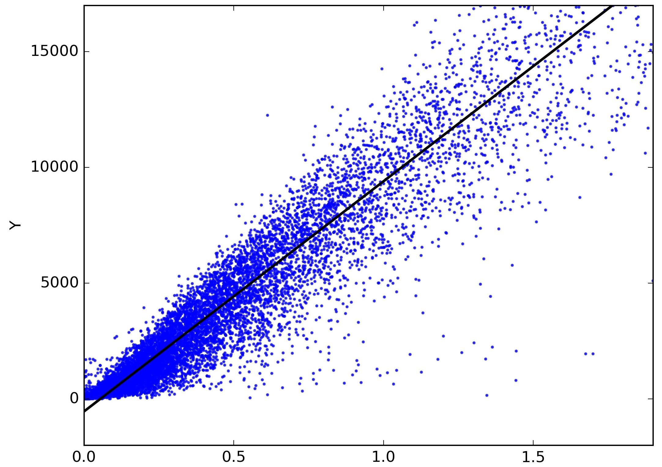
When plotting the relationship between the input variables and the target variable on a coordinate grid, a linear relationship is observed if the points form a pattern that can be approximated by a straight line. This line represents the best-fit solution that the linear model aims to find.
Linearity assumes that there are no major interactions or nonlinear effects between the input variables. If there are interactions or nonlinear relationships present in the data, the linear model may not accurately capture these complexities. It is important to assess the linearity assumption before applying a linear model to a dataset.
One way to verify linearity is by plotting a scatter plot of the input variables against the target variable. If the points follow a linear trend, it suggests a linear relationship. However, if the points deviate substantially from a straight line or exhibit a curved pattern, it indicates nonlinearity.
Furthermore, it is essential to consider the underlying domain knowledge and the nature of the problem when evaluating linearity. Some relationships may appear nonlinear at first glance but can be transformed into a linear form through appropriate feature engineering techniques.
Overall, understanding linearity is crucial for effectively applying linear models. It enables us to interpret the relationship between input and output variables accurately and make informed decisions based on the model’s predictions.
Key Components of a Linear Model
A linear model consists of several key components that work together to estimate the relationship between input variables and the target variable. Understanding these components is essential for building and interpreting linear models effectively.
1. Input Variables: Also known as independent variables or features, these are the characteristics or factors that influence the target variable. In a linear model, the input variables are represented as x1, x2, …, xn.
2. Target Variable: The target variable, also known as the dependent variable, is the variable that we want to predict or explain using the input variables. It is denoted as y in a linear model.
3. Coefficients: The coefficients, represented by b0, b1, b2, …, bn, are the weights assigned to each input variable in the linear equation. They determine the impact and direction of the relationship between the input variables and the target variable. These coefficients are estimated during the model training process.
4. Intercept: The intercept, denoted as b0, represents the estimated value of the target variable when all the input variables are zero. It is the point where the linear regression line intersects the y-axis.
5. Error Term: The error term, also known as the residual, accounts for the discrepancy between the predicted and actual values of the target variable. It represents the unexplained variation in the data that cannot be captured by the linear relationship.
6. Residuals: Residuals are the differences between the predicted values and the actual values of the target variable. Analyzing the residuals helps evaluate the accuracy of the model and identify patterns or trends that may indicate model deficiencies.
7. Assumptions: Linear models rely on several assumptions, including linearity, independence of errors, homoscedasticity (constant variance of errors), and normal distribution of errors. Violations of these assumptions may affect the validity and reliability of the model’s predictions.
By understanding and considering these key components, we can effectively interpret and evaluate a linear model’s results. They provide insights into the relationships between the variables and guide us in making informed decisions based on the model’s predictions.
Types of Linear Models
Linear models come in various forms, each with its own characteristics and strengths. Let’s explore some of the most commonly used types of linear models:
1. Simple Linear Regression: Simple linear regression is the most basic form of a linear model. It involves a single input variable and a target variable, following a linear relationship. The goal is to find the best-fit line that minimizes the difference between the predicted values and the actual values of the target variable.
2. Multiple Linear Regression: Multiple linear regression extends the concept of simple linear regression by incorporating multiple input variables to predict the target variable. It allows for more complex relationships and provides a way to account for the combined effects of multiple predictors.
3. Polynomial Regression: Polynomial regression is a type of linear regression that models the relationship between the input variables and the target variable using polynomials of different degrees. It can capture nonlinearity by introducing higher-order terms such as x^2, x^3, etc. This makes it flexible in fitting curved or nonlinear patterns in the data.
4. Ridge Regression: Ridge regression is a regularization technique used to overcome overfitting in linear models. It introduces a penalty term, the ridge term, that adds a bias to the coefficients during the model training process. This helps to reduce the impact of multicollinearity and stabilizes the model’s performance.
5. Lasso Regression: Lasso regression, short for Least Absolute Shrinkage and Selection Operator, is another regularization technique used in linear models. Similar to ridge regression, it introduces a penalty term, but in this case, it uses an absolute value rather than a square of the coefficients. Lasso regression can enforce sparsity in the model by driving some coefficients to exactly zero, effectively selecting the most important features for prediction.
6. Elastic Net Regression: Elastic Net regression combines the properties of both ridge regression and lasso regression. It introduces both the ridge term and the lasso term in the regularization process, providing a balance between feature selection and bias reduction. Elastic Net regression is particularly useful when dealing with datasets that have a large number of features and potential collinearity.
These are just a few examples of the types of linear models commonly used in machine learning and statistics. Each type has its own advantages and is suitable for different scenarios and data characteristics. Choosing the appropriate type of linear model is crucial for achieving accurate and reliable predictions.
Assumptions and Limitations of Linear Models
While linear models are widely used and have several advantages, they also rely on certain assumptions and have limitations that need to be considered. Understanding these assumptions and limitations is important for proper application and interpretation of linear models:
1. Linearity: Linear models assume a linear relationship between the input variables and the target variable. If the relationship is nonlinear, the model may not provide accurate predictions. It is crucial to assess the linearity assumption by examining scatter plots or other diagnostic techniques.
2. Independence of Errors: Linear models assume that errors or residuals are independent of each other. In other words, the errors for one observation should not be related to the errors of other observations. Violation of this assumption, such as in time-series data or spatially correlated data, can lead to biased or inefficient estimates.
3. Homoscedasticity: Homoscedasticity refers to the assumption that the variability of the errors should be constant across all levels of the input variables. If the variability of errors changes systematically with the input variables (heteroscedasticity), it can affect the accuracy of predictions and the reliability of the model.
4. Normality of Errors: Linear models assume that the errors follow a normal distribution. Deviations from normality can affect the validity of statistical tests and confidence intervals. However, linear models are robust to moderate deviations from normality, especially with large sample sizes.
5. Outliers and Influential Points: Linear models can be sensitive to outliers and influential points, which are observations that have a disproportionately large effect on the model’s fit. It is important to identify and handle these observations appropriately to avoid biased estimation.
6. Multicollinearity: Multicollinearity occurs when there is a high correlation between two or more input variables. It can lead to unstable or unreliable estimates of the coefficients and make it difficult to interpret the individual effects of the variables. Various techniques, such as feature selection and regularization, can be used to handle multicollinearity.
7. Overfitting: Linear models may suffer from overfitting, where the model becomes too complex and fits the noise in the data rather than the underlying relationships. Regularization techniques, such as ridge regression and lasso regression, can help mitigate overfitting by adding a penalty term to the model’s objective function.
8. Nonlinear Relationships: Linear models have limited flexibility in capturing nonlinear relationships between the input and target variables. If the relationship is highly nonlinear, alternative modeling techniques may be more appropriate, such as polynomial regression, spline regression, or nonlinear regression models.
Despite these assumptions and limitations, linear models remain valuable tools in various domains. Understanding their assumptions and limitations allows for informed decision-making and ensures the appropriate use of linear models in different scenarios.
Training and Evaluating a Linear Model
Training and evaluating a linear model involves several steps to ensure its effectiveness and reliability. Let’s explore the key aspects of this process:
1. Data Preparation: Start by preparing the dataset for training the linear model. This involves cleaning the data, handling missing values, and performing feature scaling if necessary. It is important to ensure that the data is in a format suitable for analysis.
2. Splitting the Data: Divide the dataset into training and testing sets. The training set is used to train the model, while the testing set is kept separate and used to evaluate its performance. Cross-validation techniques, such as k-fold cross-validation, can also be applied to obtain more robust estimates of the model’s performance.
3. Model Training: Fit the linear model to the training data by estimating the coefficients that best fit the relationship between the input variables and the target variable. This is typically done using optimization algorithms such as ordinary least squares or gradient descent.
4. Model Evaluation: Evaluate the performance of the trained linear model using appropriate evaluation metrics such as mean squared error, mean absolute error, or R-squared value. These metrics provide insights into how well the model is able to make predictions compared to the actual values. It is important to interpret these metrics in the context of the specific problem and set an acceptable threshold for model performance.
5. Interpreting Coefficients: Analyze the estimated coefficients of the linear model to understand the relationship between the input variables and the target variable. Positive coefficients indicate a positive influence on the target variable, while negative coefficients indicate a negative influence. The magnitude of the coefficients reflects the strength of the relationship.
6. Model Improvement: If the initial model performance is not satisfactory, consider improving it by incorporating feature selection techniques or regularization methods. Feature selection helps identify the most relevant features, reducing noise and improving prediction accuracy. Regularization techniques, such as ridge regression or lasso regression, can help overcome potential issues such as multicollinearity or overfitting.
7. Model Validation: Validate the final trained model using the testing set or additional validation sets. This will provide a realistic estimate of the model’s performance on unseen data. Validate the model against different metrics or consider using domain-specific evaluation criteria to ensure its suitability and reliability.
By following these steps and considering the evaluation and validation processes, you can train a robust and effective linear model. Continuously monitoring the model’s performance and making necessary adjustments will help ensure its accuracy and reliability.
Feature Selection and Engineering in Linear Models
Feature selection and engineering play a crucial role in improving the performance and interpretability of linear models. By carefully selecting relevant features and engineering new ones, we can enhance the predictive power of the model and capture important patterns in the data. Here are some key aspects of feature selection and engineering in linear models:
1. Feature Selection: It involves identifying the most informative features that have the most significant impact on the target variable. This helps reduce the dimensionality of the problem and remove unnecessary noise. Techniques such as statistical tests, correlation analysis, and stepwise regression can guide the selection of features based on their relevance and contribution to the model’s performance.
2. Domain Knowledge: It is important to incorporate domain knowledge and expertise when selecting features for a linear model. Domain knowledge can help identify key variables that are known to influence the target variable. This can lead to more accurate and meaningful predictions by including relevant factors that may not be evident from the data alone.
3. One-Hot Encoding: Categorical variables often require special handling in linear models. One-hot encoding is a technique used to convert categorical variables into a binary format, where each category is represented by a binary column. This enables the linear model to capture the effects of categorical variables without assuming any specific order or hierarchy among them.
4. Polynomial Features: Linear models assume linearity between the input and output variables. However, sometimes the relationship may be nonlinear or have higher-order interactions. In such cases, creating polynomial features by exponentiating the original features can capture the nonlinearities and improve the model’s performance. However, caution must be exercised to avoid overfitting and multicollinearity when using polynomial features.
5. Interaction Terms: Interaction terms are created by multiplying two or more input variables together. Including interaction terms in the model allows for capturing interactions and synergistic effects between variables. For example, if the effect of one feature on the target variable changes depending on the value of another feature, an interaction term can help capture this relationship.
6. Regularization and Feature Importance: Regularization techniques like ridge regression and lasso regression can automatically select and penalize the less important features, providing a built-in feature selection mechanism. By considering the magnitude of the coefficients, we can identify the most influential features and focus on interpreting their effects on the target variable.
7. Iterative Improvement: Feature selection and engineering are iterative processes. It involves continually refining the set of features based on their performance and contribution to the model’s accuracy. It may require trial and error, experimentation, and domain-specific knowledge to identify the optimal set of features that best capture the underlying relationships.
By implementing effective feature selection and engineering techniques, we can improve the performance, interpretability, and generalization capabilities of linear models. It enables us to focus on the most informative features and capture complex relationships, ultimately leading to more accurate and meaningful predictions.
Handling Nonlinearity in Linear Models
Linear models assume a linear relationship between input variables and the target variable. However, real-world datasets often exhibit nonlinear relationships that cannot be adequately captured by a simple straight line. Fortunately, there are several techniques available to handle nonlinearity in linear models:
1. Polynomial Regression: Polynomial regression is a technique that extends the linear model to capture nonlinear relationships by introducing polynomial features. By including higher order terms such as squares, cubes, or higher-degree powers of the input variables, the model can better fit data with curvature and nonlinear patterns. However, it is important to balance the complexity of the model to prevent overfitting.
2. Transformations: Transforming the input variables can help linearize nonlinear relationships. Common transformations include logarithmic, exponential, square root, or inverse transformations. These transformations can help normalize skewed data, reduce heteroscedasticity, and linearize nonlinear relationships. It is important to select appropriate transformations based on the specific distribution and characteristics of the data.
3. Splines: Splines are a flexible technique for handling nonlinearity by dividing the range of the input variable into smaller intervals and fitting a piecewise function within each interval. The points where separate functions meet are called knots. Splines can capture complex nonlinear relationships without using high-degree polynomials, reducing the risk of overfitting. Popular types of splines include cubic splines and natural splines.
4. Interaction Terms: Interaction terms capture the combined effect of two or more input variables on the target variable. By introducing interaction terms into the linear model, we can model nonlinear relationships that arise from the interaction between predictors. For example, if the effect of one variable on the target variable changes depending on the value of another variable, including their interaction term can capture this nonlinear relationship.
5. Nonlinear Transformations within Linear Models: In some cases, it is possible to incorporate nonlinear transformations within linear models through techniques such as generalized additive models (GAMs) or kernel methods. These approaches allow for the incorporation of nonlinear functions, such as spline basis functions or radial basis functions, to model the relationship between the input variables and the target variable within a linear framework.
6. Nonlinear Model Alternatives: If the nonlinearity in the data is too complex to be captured by linear models, it may be necessary to consider alternative modeling approaches, such as decision trees, random forests, support vector machines, or neural networks. These models can handle highly nonlinear relationships and interactions but may sacrifice some of the interpretability and simplicity offered by linear models.
It is important to assess the type and degree of nonlinearity in the data when choosing the appropriate technique for handling nonlinearity in a linear model. Each approach has its strengths and limitations, and the choice should be based on the specific dataset, the desired interpretability, and the objectives of the analysis.
Regularization Techniques in Linear Models
Regularization techniques are commonly used in linear models to prevent overfitting and improve the model’s generalization performance. These techniques add a regularization term to the objective function, which helps control the complexity of the model. Here are some popular regularization techniques used in linear models:
1. Ridge Regression: Ridge regression, also known as Tikhonov regularization, adds a penalty term to the least squares objective function. This penalty term is proportional to the square of the coefficients, which discourages large coefficients. By adding this regularization term, ridge regression reduces model complexity and handles the issue of multicollinearity by shrinking the coefficients towards zero. The strength of regularization in ridge regression is controlled by the regularization parameter, also known as lambda or alpha.
2. Lasso Regression: Lasso regression, short for Least Absolute Shrinkage and Selection Operator, is similar to ridge regression but uses the absolute value of the coefficients instead of their squares as the penalty term. This promotes sparsity in the model by driving some coefficients exactly to zero. Lasso regression not only reduces model complexity but also performs feature selection by automatically excluding less relevant features. The regularization strength in lasso regression is also controlled by the regularization parameter.
3. Elastic Net Regression: Elastic Net regression combines both ridge regression and lasso regression techniques. It adds a linear combination of both the L1 norm (lasso penalty) and the L2 norm (ridge penalty) to the objective function. Elastic Net regression overcomes the limitations of ridge regression and lasso regression by providing a balance between feature selection and parameter shrinkage. The regularization strength in elastic net regression is controlled by two parameters: alpha, which controls the regularization mix, and lambda, which controls the overall regularization strength.
4. Decision Threshold: In addition to regularized regression techniques, decision thresholds can be set to filter or eliminate coefficients that fall below a certain threshold. This acts as a regularization technique by removing less important features and simplifying the model.
Regularization techniques help prevent overfitting in linear models by reducing the impact of irrelevant or highly correlated features. They encourage models to generalize well to unseen data and improve the model’s stability and performance. The choice between ridge regression, lasso regression, or elastic net regression depends on the specific data characteristics, the importance of feature selection, and the desired balance between parameter shrinkage and sparsity in the model.
Real-World Applications of Linear Models
Linear models find extensive use in a wide range of real-world applications, thanks to their simplicity, interpretability, and effectiveness. Here are some examples of how linear models are applied in different domains:
1. Finance and Economics: Linear models are widely used in finance and economics for various purposes. They help analyze stock price trends, predict market volatility, and model financial risk. Linear regression can be employed to understand the relationship between economic indicators, such as interest rates or inflation, and their impact on investments or consumer behavior.
2. Marketing and Sales: Linear models play a crucial role in marketing and sales analytics. They are instrumental in customer segmentation, determining pricing strategies, and predicting customer lifetime value. Linear regression models can be used to identify influential marketing channels, assess the impact of advertising campaigns, or optimize marketing spend allocation.
3. Healthcare: Linear models have applications in healthcare as well. They are used to predict patient outcomes based on various clinical factors, such as age, medical history, and vital signs. Linear regression can also be employed to study the impact of a specific treatment or intervention on patient outcomes and medical costs.
4. Social Sciences: In social sciences, linear models are used to study and understand human behavior. They can help investigate the relationship between socio-economic factors and educational attainment, analyze survey data, or predict voting patterns based on demographic information. Linear models aid in explaining and predicting various aspects of human behavior.
5. Environmental Science: Linear models are utilized in environmental science to analyze climate data, understand the impact of pollution on ecosystems, and predict natural phenomena. They can be used to study the relationship between temperature, rainfall, and ecological changes, aiding in environmental conservation and decision-making.
6. Engineering: Linear models find application in various branches of engineering. They help optimize processes, analyze the impact of different design variables, and predict equipment failure rates. Linear regression models can be used in fields such as mechanical engineering, civil engineering, and industrial engineering to improve performance and reliability.
7. Sports Analytics: Linear models are increasingly used in sports analytics to gain insights into player performance, team dynamics, and game strategies. They help predict player performance based on various variables such as historical data, physical attributes, and opponent analysis. Linear regression can also be used to assess the impact of different factors on team success.
These examples illustrate the versatility and practicality of linear models across various domains. Their simplicity and interpretability make them valuable tools for extracting insights, making predictions, and aiding decision-making in real-world applications.