
Understanding Categorical Data
Categorical data is a type of data that represents the specific groups or categories to which an observation belongs. It can take on a limited number of distinct values, called levels, which represent different categories or classes. Unlike numerical data, categorical data cannot be ordered or measured on a continuous scale.
Categorical data is commonly encountered in various fields such as market research, social sciences, and machine learning. Examples of categorical data include gender (male or female), colors (red, blue, green), and education level (elementary, high school, college).
Understanding the nature of categorical data is crucial for effectively analyzing and interpreting it. It is important to note that categorical data can be further classified into nominal and ordinal data.
Nominal data refers to categories that have no inherent order or ranking. For example, the colors of a car (red, blue, green) or the breeds of dogs (Labrador, German Shepherd, Bulldog) are nominal categorical variables.
On the other hand, ordinal data represents categories with a clear ordering or ranking. For instance, education level (elementary, high school, college) or customer satisfaction ratings (very satisfied, satisfied, neutral, dissatisfied) are examples of ordinal categorical variables. In ordinal data, the relative order of the categories matters, as they express a certain level of significance or hierarchy.
Understanding the type of categorical data you’re dealing with is essential to select the appropriate techniques for data preprocessing and feature engineering. Various encoding methods, such as one-hot encoding, label encoding, and ordinal encoding, can be utilized to convert categorical data into a numerical format that machine learning algorithms can process effectively. Additionally, strategies for handling missing values and rare categories need to be considered when working with categorical data.
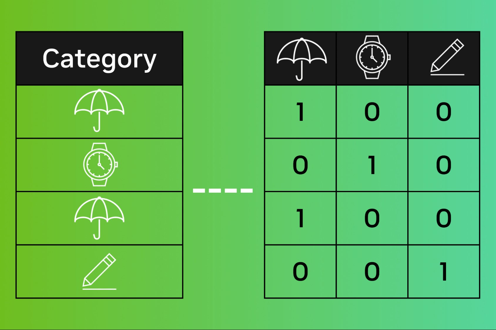
One-Hot Encoding
One-hot encoding is a popular technique used to convert categorical variables into a numerical format that can be easily understood and processed by machine learning algorithms. It creates binary features for each category in a variable, indicating the presence or absence of that category.
To illustrate this technique, consider a variable like “color” with three categories: red, blue, and green. One-hot encoding would create three new binary variables: “color_red”, “color_blue”, and “color_green”. Each variable would have a value of 1 if the original observation belongs to that category, and 0 otherwise.
This method ensures that all information contained in the categorical variable is preserved without assigning any ordinal relationship between the categories. However, it can lead to the problem of high dimensionality in datasets with many distinct categories. Therefore, it should be used judiciously, especially when dealing with variables with a large number of unique categories.
One-hot encoding is widely supported by machine learning libraries and frameworks. Many algorithms, such as logistic regression and decision trees, can handle this type of encoding without any issues. However, it is important to note that some algorithms, like linear regression, may encounter multicollinearity issues due to the high correlation between the binary variables created by one-hot encoding. In such cases, feature selection or dimensionality reduction techniques may be required.
Implementing one-hot encoding in Python is straightforward using libraries such as scikit-learn or pandas. These libraries offer methods like `get_dummies()` or `OneHotEncoder()` that can be applied to categorical variables. It is important to encode the categorical variables before training the machine learning model to ensure all the features are in a numerical format.
One-hot encoding is a versatile and widely-used technique for handling categorical variables in machine learning tasks. It allows algorithms to effectively process and utilize the information contained in these variables. However, it is crucial to consider the potential impact on dimensionality and choose encoding techniques that best suit the specific dataset and modeling goals.
Label Encoding
Label encoding is another method for converting categorical variables into a numerical format. Unlike one-hot encoding, which creates binary features for each category, label encoding assigns a unique numerical label to each unique category in a variable.
To illustrate the concept, let’s consider a variable like “fruit” with categories: apple, banana, and orange. Label encoding would assign the labels 0, 1, and 2 to these categories, respectively. This encoding allows machine learning algorithms to understand and process the categorical data as numerical values.
One advantage of label encoding is that it maintains the ordinal relationship between the categories. In scenarios where categories have a natural order or hierarchy, such as low, medium, and high, label encoding can provide valuable information to the algorithms. However, it is important to note that label encoding should not be applied to nominal variables, as it may introduce unintended ordinal information that does not exist.
It is essential to consider the potential pitfalls of label encoding. For instance, some algorithms may incorrectly interpret the encoded labels as meaningful numerical features, leading to erroneous assumptions about the relationship between the categories. To address this issue, additional preprocessing steps, such as one-hot encoding or target encoding, can be implemented to convert the label-encoded variables into a more suitable format for specific algorithms.
In Python, label encoding can be easily implemented using libraries such as scikit-learn or pandas. The `LabelEncoder()` class in scikit-learn and the `LabelEncoder()` method in pandas can be used to perform label encoding. These libraries provide flexible options for encoding categorical variables and integrating them into machine learning workflows.
Label encoding is a simple and effective technique for transforming categorical variables into numerical format. It is particularly useful for variables with an inherent order or hierarchy. However, it is crucial to be mindful of the potential impact on algorithms and to appropriately preprocess and transform the encoded variables to achieve optimal results in machine learning tasks.
Ordinal Encoding
Ordinal encoding is a categorical variable encoding technique that assigns numerical labels to categories based on their ordinal relationship or natural order. It is particularly useful when dealing with categorical variables that exhibit a clear hierarchy or ranking.
To perform ordinal encoding, we assign increasing integers to the categories in an ordered manner. For example, if we have a variable called “education level” with categories “elementary,” “high school,” and “college,” we can assign labels 0, 1, and 2 to these categories, respectively. Ordinal encoding preserves the ordinal relationship between the categories and allows machine learning algorithms to take advantage of this information.
Ordinal encoding is a sensible choice when the order of categories carries some meaning or impact on the outcome. For example, in a sentiment analysis task with categories like “negative,” “neutral,” and “positive,” ordinal encoding can represent the sentiment intensity effectively.
However, it is important to exercise caution when applying ordinal encoding to variables with no clear order or when the chosen order might introduce unintended ordinal assumptions. In such cases, using label encoding or one-hot encoding may be more appropriate.
In Python, ordinal encoding can be implemented using libraries such as scikit-learn or pandas. The `OrdinalEncoder()` class in scikit-learn and the `replace()` method in pandas are commonly used for this purpose. These libraries offer flexibility in handling various encoding scenarios and integrating the encoded variables into machine learning workflows.
It is worth mentioning that ordinal encoding, like label encoding, may not be suitable for all machine learning algorithms. Some algorithms may interpret the encoded labels as meaningful numerical features and make assumptions about the magnitude or distance between the categories. Consequently, it is crucial to evaluate the compatibility of ordinal encoding with the chosen algorithm and explore alternative encoding techniques if necessary.
Ordinal encoding is a valuable encoding technique when working with categorical variables that exhibit a clear hierarchy or ranking. By preserving the ordinal relationship, it enables the machine learning algorithm to capture the inherent order of the categories. Nevertheless, careful consideration must be given to the nature of the variable and the assumptions made by the algorithm to ensure accurate and meaningful results in machine learning tasks.
Binary Encoding
Binary encoding is a categorical variable encoding technique that converts categories into binary code. It is a space-efficient alternative to one-hot encoding that can effectively represent categorical variables with a large number of distinct categories.
Binary encoding works by first assigning a unique integer value to each category. Then, the integer value is converted into binary code. Each binary digit represents a bit, with 0 indicating the absence of a category and 1 indicating its presence. The number of binary digits required is determined by the logarithm base 2 of the number of unique categories. For example, if we have 4 distinct categories, we would need 2 binary digits (2^2 = 4) to represent them.
Binary encoding offers several advantages. It allows for efficient memory usage, as the binary representation requires fewer bits than one-hot encoding. Moreover, it preserves some information about the ordinal relationships between categories, as the binary digits represent different powers of 2.
However, it is worth noting that binary encoding is not suitable for variables with high cardinality, as the number of required binary digits can quickly become large. In such cases, alternative encoding techniques like frequency encoding or target encoding may be more appropriate.
In Python, binary encoding can be implemented using libraries such as category_encoders or feature-engine. These libraries provide convenient functions and classes for applying binary encoding to categorical variables. Additionally, scikit-learn’s LabelBinarizer class can also be used for binary encoding, although it requires converting the categorical variable to a numerical representation first.
It is important to consider the implications of binary encoding on machine learning algorithms. While most algorithms can handle binary-encoded variables without issue, certain algorithms may struggle with high dimensionality if the number of binary digits is large. In such cases, feature selection or dimensionality reduction techniques may be necessary to mitigate the impact.
Binary encoding is a useful alternative to one-hot encoding when dealing with categorical variables with a large number of distinct categories. It offers memory efficiency and preserves some ordinal information. However, it should be used judiciously, especially when the cardinality of the variable is high, and consideration should be given to the compatibility with the chosen machine learning algorithm.
Count Encoding
Count encoding is a powerful categorical variable encoding technique that replaces each category with the count of occurrences of that category in the dataset. It assigns a numerical value to each category based on its frequency, providing valuable information to machine learning algorithms.
Count encoding is particularly useful when dealing with categorical variables with high cardinality, as it captures the relationship between the category and the target variable. By encoding categories based on the frequency of their occurrence, count encoding implicitly captures the importance or relevance of each category in the dataset.
To perform count encoding, we compute the number of occurrences of each category in the dataset and replace the category with that count. For example, if we have a categorical variable “color” with categories “red”, “blue”, and “green”, and “red” occurs 100 times, “blue” occurs 50 times, and “green” occurs 75 times, we would replace “red” with 100, “blue” with 50, and “green” with 75.
Count encoding can be easily implemented in Python using libraries such as category_encoders or feature-engine. These libraries provide convenient functions and classes that enable count encoding for categorical variables.
One of the major advantages of count encoding is that it handles high-cardinality variables effectively. Rather than creating a large number of binary variables (as in one-hot encoding) or assigning arbitrary numerical labels (as in label encoding), count encoding leverages the frequency information to represent the categories. This can be particularly helpful in cases where the rare categories are valuable or significant.
However, it is important to be cautious when dealing with categories that have not been observed in the training dataset, especially in situations where new and unseen categories may be encountered during the model’s deployment. In such cases, appropriate handling of unseen categories, such as assigning them a default count or encoding them separately, is necessary.
Count encoding is a versatile technique that captures the frequency-based information of categorical variables. By providing a numerical representation based on occurrence counts, it enables machine learning algorithms to leverage the underlying relationships between categories and the target variable. Nevertheless, careful consideration should be given to the handling of unseen categories and the potential impact on the chosen algorithm.
Target Encoding
Target encoding, also known as mean encoding or likelihood encoding, is a categorical variable encoding technique that replaces categories with the average value of the target variable for each category. It leverages the target variable’s relationship with categorical features, providing valuable information to machine learning algorithms.
Target encoding is particularly useful when dealing with categorical variables that have a strong correlation with the target variable. By encoding categories based on the target variable’s average value for each category, target encoding conveys the category’s predictive power or influence on the target.
To perform target encoding, we calculate the average value of the target variable for each category and replace the category with that average. For example, if we have a categorical variable “color” with categories “red”, “blue”, and “green”, and the average values of the target variable for these categories are 0.35, 0.45, and 0.60, respectively, we would replace “red” with 0.35, “blue” with 0.45, and “green” with 0.60.
Target encoding can be easily implemented in Python using libraries such as category_encoders or feature-engine. These libraries provide functions and classes specifically designed for target encoding categorical variables.
One of the major advantages of target encoding is its ability to capture the relationship between categorical variables and the target variable. By replacing categories with mean target values, target encoding provides a direct encoding of the predictive power of each category. This can be particularly useful in cases where there is a strong correlation between the categories and the target variable.
However, it is important to be aware of potential overfitting when applying target encoding. If the target encoding is calculated based on the entire dataset, it can lead to data leakage and cause the model to perform poorly on new, unseen data. To mitigate this, techniques such as cross-validation can be used to calculate target encodings on the training set only and then apply them to the validation or test set.
Target encoding is a powerful technique that captures the relationship between categorical variables and the target variable. By encoding categories based on the target variable’s average value for each category, it provides valuable information to machine learning algorithms. Nevertheless, proper precautions should be taken to prevent overfitting and ensure accurate model performance on new data.
Feature Hashing
Feature hashing, also known as the hash trick, is a technique used to convert categorical variables into a fixed-length representation, typically a numeric vector. It is particularly useful when dealing with high-dimensional or high-cardinality categorical data where traditional encoding techniques may become computationally expensive or memory-intensive.
The process of feature hashing involves applying a hash function to each category in a categorical variable and mapping it to a fixed number of dimensions or buckets. The resulting numeric vector represents the presence or absence of each category. The hash function ensures that different categories are well distributed across the dimensions, reducing the likelihood of collisions or duplicate hash values.
Feature hashing offers several advantages. Firstly, it allows for efficient memory usage since the resulting vector has a fixed length regardless of the number of unique categories. Secondly, it can handle high-cardinality variables efficiently by preventing the need to create a large number of binary variables, as in one-hot encoding. Finally, feature hashing allows for fast computation, making it suitable for online or streaming data processing scenarios.
One potential drawback of feature hashing is the potential for hash collisions, where different categories are mapped to the same hash value. This can result in loss of information and impact the accuracy of the model. However, by choosing an appropriate number of dimensions or adjusting the hash function, the likelihood of collisions can be minimized.
In Python, feature hashing can be implemented using libraries such as scikit-learn or the built-in hash functions in Python. The scikit-learn library provides the `FeatureHasher` class that can be used to perform feature hashing on categorical variables.
It is important to note that feature hashing may not be suitable for all scenarios. For datasets with highly informative categories or strong relationships between categories and the target variable, other encoding techniques like target encoding or count encoding may provide better results. Additionally, feature hashing may not preserve the interpretability of the original categories since the transformed features are represented in a numeric format.
Feature hashing is a versatile technique for encoding high-dimensional or high-cardinality categorical variables. By converting categories into a fixed-length representation, it offers memory efficiency and computational speed advantages. However, careful consideration should be given to the potential impact of collisions and the interpretability of the transformed features in relation to the original categories.
Frequency Encoding
Frequency encoding, also known as count encoding, is a technique used to encode categorical variables by replacing each category with its frequency or count within the dataset. It assigns a numerical value to each category based on its occurrence frequency, providing valuable information to machine learning algorithms.
To perform frequency encoding, we compute the number of occurrences of each category in the dataset and replace the category with that count. For example, if we have a categorical variable “color” with categories “red”, “blue”, and “green”, and “red” occurs 100 times, “blue” occurs 50 times, and “green” occurs 75 times, we would replace “red” with 100, “blue” with 50, and “green” with 75.
Frequency encoding can be easily implemented in Python using libraries such as category_encoders or feature-engine. These libraries provide functions and classes specifically designed for frequency encoding categorical variables.
Frequency encoding offers several advantages. Firstly, it captures the relationship between the categorical variable and the target variable indirectly, as the frequency of a category can be correlated with the target variable. Secondly, it handles high-cardinality variables efficiently, as no additional memory or computational resources are required to encode them. Finally, frequency encoding can be useful in situations where rare categories are valuable or meaningful, as they will have lower frequency values.
However, it is important to be cautious when applying frequency encoding, especially with high-dimensional datasets, as categories with low frequencies can introduce noise or overfitting. To mitigate this, smoothing techniques, such as Laplace smoothing or target-based smoothing, can be employed to balance the encoding and prevent extreme values.
It is worth noting that frequency encoding may not be suitable for all scenarios. In cases where there is no inherent ordering or hierarchy among the categories, techniques like one-hot encoding or label encoding may be more appropriate. Additionally, frequency encoding may not preserve the interpretability of the original categories since they are transformed into numerical frequency values.
Frequency encoding is a powerful technique for encoding categorical variables based on their frequency of occurrence in the dataset. By assigning numerical values to categories, it provides valuable information to machine learning algorithms and can handle high-cardinality variables efficiently. However, careful consideration should be given to smoothing techniques and the interpretability of the transformed features in relation to the original categories.
Handling Imbalanced Categories
Imbalanced categories refer to categorical variables where the distribution of categories is significantly skewed or unbalanced. This can pose challenges in machine learning tasks as it may lead to biased models that prioritize the majority categories, resulting in poor performance on the minority categories. Handling imbalanced categories is crucial to ensure fair representation and accurate predictions across all categories.
There are several techniques for addressing imbalanced categories. One common approach is oversampling, which involves replicating or generating synthetic samples from the minority categories to achieve a balance with the majority categories. This can be done using methods like Random Oversampling, SMOTE (Synthetic Minority Over-sampling Technique), or ADASYN (Adaptive Synthetic Sampling).
Another approach is undersampling, which involves reducing the number of samples from the majority categories to match the number of samples in the minority categories. This can be achieved using methods like Random Undersampling or Cluster Centroids.
A more advanced technique is using ensemble methods specifically designed for imbalanced categories, such as Balanced Random Forest or EasyEnsemble. These methods account for class imbalance by resampling the data or adjusting the algorithm’s parameters to give more weight to the minority classes.
Moreover, incorporating class weights during model training can help address imbalanced categories. Class weights assign higher weights to samples from the minority categories, allowing the algorithm to pay greater attention to these categories during training.
Lastly, it is important to choose suitable evaluation metrics when dealing with imbalanced categories. Metrics such as precision, recall, F1-score, and area under the ROC curve (AUC-ROC) provide a more comprehensive understanding of model performance when categories are imbalanced. By focusing on these metrics, we can better assess the model’s ability to accurately classify samples across all categories.
When handling imbalanced categories, it is necessary to carefully consider the potential impact of each technique and evaluate its effectiveness on the specific dataset and machine learning algorithm being used. Additionally, it is important to validate the performance of the model on unseen data to ensure its generalizability.
In summary, imbalanced categories can present challenges in machine learning tasks, but there are various techniques available to address the issue. By applying appropriate oversampling, undersampling, ensemble methods, or adjusting class weights, we can ensure fair representation and accurate predictions across all categories. Moreover, using suitable evaluation metrics is crucial for assessing model performance in the presence of imbalanced categories.
Dealing with Missing Values in Categorical Data
Missing values in categorical data can occur due to various reasons, such as data collection errors or incomplete information. It is essential to properly handle missing values before proceeding with any analysis or modeling, as they can impact the accuracy and validity of results. Here are some common approaches to dealing with missing values in categorical data.
1. Dropping Rows or Columns: If the missing values are minimal and occur randomly, one straightforward solution is to remove the rows or columns containing missing values. However, this method should be used cautiously, as it may result in loss of valuable data and potentially biased results if the missingness is not random.
2. Filling with Mode: For categorical variables, the mode represents the most frequent category. Filling missing values with the mode is a simple and common approach, especially when the missingness occurs in a small proportion of the data. However, this method assumes that the missing values are missing completely at random (MCAR) or missing at random (MAR).
3. Creating a New Category: In some cases, it may be appropriate to create a new category or label to represent missing values. This can be useful when the missingness itself carries some information or when the missing values constitute a large proportion of the data. By introducing a unique category for missing values, the model can potentially learn from this information.
4. Imputation based on Other Features: If there are other related features available, missing values in a categorical variable can be imputed based on the values of other features. This can involve using techniques such as k-nearest neighbors imputation, which finds the nearest neighbors based on other features and imputes the missing values with the most common category among those nearest neighbors.
5. Using Predictive Models: Predictive models can be used to impute missing values in categorical data. For example, decision tree-based algorithms like random forests or gradient boosting can be trained on the available data to predict the missing values based on the values of other features. The predicted values can then be used for imputation.
When dealing with missing values in categorical data, it is crucial to carefully consider the reasons for the missingness, the proportion of missing values, and the impact on the analysis or modeling task. Additionally, it is important to perform sensitivity analysis to understand the potential effects of different imputation methods on the results.
In summary, there are various techniques available for handling missing values in categorical data. The choice of method depends on factors such as the extent of missingness, the underlying causes, and the goals of the analysis or modeling task. By appropriately addressing missing values, we can ensure the integrity and reliability of the results obtained from categorical data analysis.
Feature Selection with Categorical Data
Feature selection is a crucial step in machine learning, as it helps identify the most relevant and informative features for building models. When working with categorical data, selecting the right set of features becomes essential to optimize model performance and interpretability. Here are some techniques for feature selection specifically tailored for categorical data.
1. Chi-squared Test: The chi-squared test is a statistical method that can assess the independence between a categorical target variable and each categorical feature. By calculating the chi-squared statistic and corresponding p-value, we can determine the significance of the relationship. Features with a significant relationship to the target variable can be selected for further analysis or modeling.
2. Information Gain: Information gain, based on the concept of entropy, is a measure of the reduction in uncertainty achieved by including a particular feature in the model. Higher information gain values indicate more predictive power of the feature. Decision tree-based algorithms, such as entropy-based decision trees or random forests, can be used to calculate the information gain of each feature, enabling feature selection based on this criterion.
3. Feature Importance from Tree-Based Models: Tree-based models, such as random forests or gradient boosting machines, provide feature importance scores that quantify the contribution of each feature in the model’s performance. These scores can be utilized to rank and select the most important features. By considering only the top-ranked features, we can reduce dimensionality and potentially enhance model performance.
4. Recursive Feature Elimination (RFE): RFE is an iterative feature selection technique that first trains a model with all features and repeatedly eliminates the least important feature until a predefined number of features remains. This technique can be applied with various machine learning algorithms, such as logistic regression or support vector machines, to identify the most relevant features while considering the interaction between features.
5. L1 Regularization: L1 regularization, also known as Lasso regularization, can be used with linear models to shrink the coefficients of less relevant features to zero. This process effectively performs feature selection by excluding features with zero coefficients, resulting in a sparse model. L1 regularization can be particularly useful when multicollinearity exists among features.
A combination of these techniques can be applied for robust feature selection with categorical data. It is important to consider the specific characteristics of the dataset, the modeling algorithm being used, and the desired balance between model performance and interpretability.
Additionally, domain knowledge and expert intuition can play a valuable role in feature selection. Understanding the context and relationships between variables can guide the selection of relevant features and help in building more accurate models.
In summary, feature selection is a critical step when working with categorical data. Through techniques like chi-squared test, information gain, feature importance, RFE, and L1 regularization, we can identify and retain the most informative features while reducing dimensionality. By selecting the right set of features, we can improve model performance, interpretability, and overall data analysis tasks.
Handling Rare Categories
Rare categories in categorical variables refer to categories that have a low frequency or occurrence within the dataset. Handling rare categories is important in machine learning tasks as they can lead to sparse data, unreliable models, and biased predictions. Here are some techniques for effectively handling rare categories.
1. Grouping as ‘Other’: One simple approach is to group rare categories into a single ‘Other’ category. By combining infrequent categories, we can reduce the sparsity in the data and prevent overfitting to rare categories. This technique works well when the rare categories share similar characteristics or have little predictive value individually.
2. Frequency-based Threshold: Another approach is to define a threshold based on the desired frequency or percentage of occurrence. Categories with frequencies below the threshold are considered rare and can be grouped together or treated as a special category. The threshold can be determined based on the dataset’s characteristics and modeling goals.
3. Target Encoding: Target encoding can be useful in handling rare categories by incorporating the target variable information. By encoding the rare categories with the target variable’s average value, we provide a more reliable estimate of their predictive power. This can help in capturing the underlying relationships between rare categories and the target variable.
4. Rare Category Replacement: Rare category replacement involves replacing the rare categories with a more general category or a category with similar characteristics. This helps avoid the sparsity issue and allows the model to generalize patterns from similar categories. The replacement category can be determined based on domain knowledge or clustering techniques.
5. One-Hot Encoding with Threshold: One-hot encoding can be adjusted by considering a threshold for rare categories. Instead of one-hot encoding all categories, only the categories above the threshold are encoded as binary features. The rare categories are grouped together or assigned a separate ‘Other’ feature.
When deciding how to handle rare categories, it is important to strike a balance between preserving relevant information and managing the data sparsity issue. Domain knowledge, insight into the dataset, and the specific modeling task play a crucial role in making informed decisions about the appropriate technique to use.
Additionally, it is important to validate the impact of handling rare categories on the model’s performance through rigorous evaluation and testing. This ensures that the chosen approach improves the model’s generalizability and does not introduce any unintended biases.
In summary, handling rare categories is essential in categorical data analysis. By grouping rare categories, determining thresholds, using target encoding, replacing rare categories, or adjusting one-hot encoding, we can mitigate the issues associated with rare categories and build more reliable and accurate models. The choice of technique depends on the dataset’s characteristics, the modeling goals, and the level of domain knowledge available.